Create professional looking spreadsheet layouts with additional formatting
Format rows or columns
Add rows or columns
To add a row or column, right-click on the row or column next to where you want your row or column to be, then click Insert or Add (depending on your program). Select whether it's a row or column you are after, and if it's either above or below, left or right to the area where you clicked. You can also navigate to Insert, and select the appropriate action.
Delete rows or columns
There are even fewer clicks for this! Right-click on the row or column you want to delete, then select Delete row or Delete column. Alternatively, you can navigate to Edit, and select the appropriate action.
Add headers
To create an easy to read table, a good start, which isn't really optional, is to add column headers to your data. To add headers to your worksheet, add the description of the values in the first row of each column.
You can change the size of the cell, the size of the text, and the colors to make them look more like titles of each column.
Add alternating colors
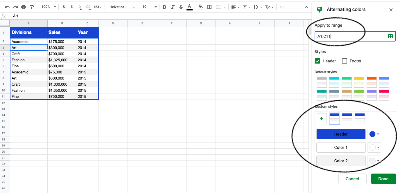
You can also format a selection of cells automatically so that they look more like a presentable table. The quickest way to accomplish this is to navigate to Format in the main menu bar, then Alternating Colors.
As shown in the image below, designating a header creates a difference between the first row and the subsequent ones. Through formatting, you can have alternating colors, or simply make them all one shade if there’s no reason to alternate colors. You can customize this to your liking and brand colors.
Change sizes of cells
Change the size of cells by hovering over the letters ( A, B, C, D ...) in the horizontal axis and the numbers in the vertical axis ( 1, 2, 3, 4 ...) of your spreadsheet. Wait for an arrow to appear, and you'll be able to drag the cell to the size you'd like.
Right-clicking works too!
Change colors or fonts
Format colors and fonts with these buttons:

Here is a recap of everything you can do with these buttons:
Font | Click the down arrow for available fonts. |
Size | Click the down arrow next to the number for available sizes. |
Weight and look of the font | Click the option to bold, italicize, or strikethrough. This can also be accomplished in the Format menu. |
Color of the font | Click the button with the underlined A. |
Filling the cell background with color | Click the pouring paint bucket. |
Edit gridlines
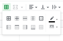
If you want to format borders, click the four squares or grid button:
If you want to delete gridlines altogether so the background looks like a blank page, you can do this too. In this case, navigate to View, and deselect Gridlines.
Freeze column or row
Freezing rows and columns makes for a better reader experience. When there’s a lot of data, it’s hard to remember what you read in the first column or first row. Freezing columns and rows allows the reader a reference to what they’re reviewing. To freeze a row or a column, navigate to View > Freeze , then select the row or column.
Each spreadsheet program may have a limit on the number of rows or columns that can be frozen. However, generally only the first few rows are frozen.
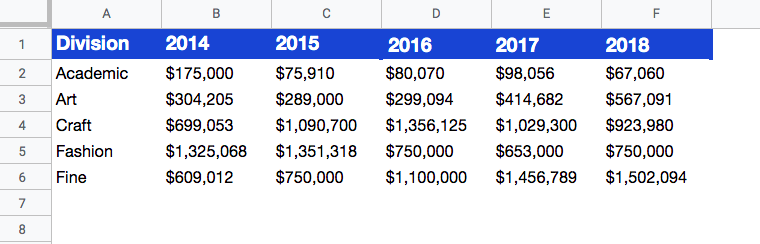
Here is a quick demo of a first row and column being frozen:
Merge cells
From time to time, you may want to merge cells. Your spreadsheet presentation will look better and not disrupt the readability of the values in other cells within the spreadsheet.
To merge cells, you select the range of cells you would like to merge, and navigate to Format > Merge cells. You can also use the following quick action button.

Here is a demo of how you can merge, with words of caution along the way.
Align the contents of a cell
Just like you would align text in a word document to standardize how it looks on a page, you can align the contents of your cell to the right, left, or center.
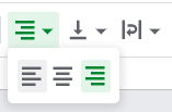
But in a spreadsheet, you can also decide whether you want to align the contents at the top, bottom, or center of a cell.
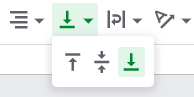
All of these alignment features can also be accessed through the Format , then Align option in the dropdown.
Wrap the contents of a cell
The quick action button to wrap content around a cell (so that the content fits into it) is one over from the two alignment ones mentioned above.
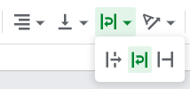
You have two other options on either side: overflow and clip, but this cuts off text. You generally want to either wrap or make the size of your columns or rows wider, so the content isn't cut off for the reader. Remember, formatting is all about making things readable!
Again, you can access this from the Format option in the menu too, by clicking there and then on Text Wrapping.
Let’s recap!
There are a lot of formatting options, and they are all meant to help make the spreadsheet look more professional and help the audience read the relevant data.
Colors, fonts, and sizes are essential to make data stand out or add a bit of design to the contents, but make sure to not overuse any of these formatting options. Keep it simple.
Merging cells can help the audience read the spreadsheet.
Freezing rows and columns make for a better reading experience because they can relate the data to the header.
Aligning and wrapping are good formatting tools, and it's important to use them consistently within the same sheet and ideally from one tab to another.
Now that we’ve learned how to format the layout, we’ll spend some time learning about conditional formatting to help our data pop off the page.
