Appreciate Ordinary Least Square and Maximum Likelihood Estimation
At this point in the course, you understand how to build, interpret, and select regression models. You can also verify that linear regression is adapted to the dataset by verifying the five assumptions from the last chapter.
However, you still don't know how the coefficients of the linear regression method are calculated and why you need to satisfy these five assumptions. To understand the mechanisms behind regression modeling, you need to have a good grasp of the mathematical aspects of the method.
At the end of this chapter, you should have a good understanding of the following:
How the linear regression coefficients are calculated with both OLS and MLE.
The fundamental differences between the OLS and the MLE method.
Where the log-likelihood statistic come from.
The concept of loss function.
This chapter is more formal and mathematical than the previous ones. To make it more palatable, we will sacrifice some mathematical rigor. We will also mostly restrict ourselves to the univariate case.
Overview
There are several ways to calculate the optimal coefficients for a linear regression model. Here we focus on the ordinary least square (OLS) method and the maximum likelihood estimation (MLE) method.
The ordinary least square (OLS) method is tailored to the linear regression model. If the data is not too weird, it should always give a decent result. The OLS method does not make any assumption on the probabilistic nature of the variables and is considered to be deterministic.
The maximum likelihood estimation (MLE) method is a more general approach, probabilistic by nature, that is not limited to linear regression models.
The cool thing is that under certain conditions, the MLE and OLS methods lead to the same solutions.
The Context
Let's briefly reiterate the context of univariate linear regression. We have an outcome variable , a predictor , and samples. and are -sized vectors. We assume that there's a linear relation between and . We can write:
Where is a random variable that introduces some noise in the dataset, is assumed to follow a normal distribution with mean = 0.
The goal is to find the best coefficients and such that the estimation is as close as possible to the real values . In other words, to minimize the distance between and for all samples i.
We can rewrite that last equation as a product of a vector of coefficients and a design matrix of predictors
Where and is the 2 by N design matrix defined by:
What's important here is that:
We want and to be as close as possible.
can be written as , a product of a vector of coefficient and a matrix of samples.
The OLS Method
When we say we want the estimated values to be as close as possible to the real value , this implies a notion of distance between the samples. In math, a good reliable distance is a quadratic distance.
In two-dimensions, if the points have the coordinates and , then the distance is given by:
Our goal is to minimize the quadratic distance between all the real points and the inferred points .
And the distance between and is:
To find the value of that minimizes that distance, take the derivative of with respect to , and solve the equation:
Easy Peasy? :euh:
We'll skip the corny details of that derivation (it's online somewhere), and instead fast-forward to the solution:
And that's how you calculate the coefficients of the linear regression with OLS. :magicien:
Univariate Case
In the univariate case with N samples, the problem comes down to finding and that best solve a set of N equations with two unknowns:
The solution to this set of N equations is given by:
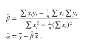
Where and are respectively the means of x and y.
Too Good to Be True?
Although it may seem that the OLS method will always output meaningful results, this is unfortunately not the case when dealing with real-world data. In the multivariate case, the operations involved in calculating this exact OLS solution can sometimes be problematic.
Calculating the matrix involves many operations including inverting the by matrix . For large number of samples , big datasets, this matrix can become huge, and inverting huge matrices takes time and large amounts of memory. Even though this large matrix inversion problem is greatly optimized today, using the closed-form solution given by the OLS method is not always the most efficient way to obtain the coefficients.
The feasibility of calculating the closed-form solution is what drives the five assumptions of linear regression.
For example, it can be shown that if there is perfect multicollinearity between the predictors (one predictor is a linear combination of the others), then the normal matrix has no inverse, and the coefficients cannot be calculated by the OLS method.
OLS Recap
What's important to understand and remember about the OLS method:
The OLS method comes down to minimizing the squared residuals.
There is a closed-form solution.
Being able to calculate this exact solution is what drives the five assumptions of linear regression.
The exact solution is difficult to calculate for a large number of samples.
Let's turn our attention now to the second method for calculating the regression coefficients, the maximum likelihood estimation, or MLE.
Maximum Likelihood Estimation (MLE)
Let's look at the problem of calculating the best coefficients of linear regression differently with this or any kind of model. The model has a potential set of parameters that best approaches a given dataset. You want to find this set of optimum parameters.
You want to maximize the probability of observing your dataset, given the parameters of that model.
In other words, find the parameters of the model that makes the current observation most likely. This is called maximizing the likelihood of the dataset.
How do we define the likelihood mathematically?
Consider the probability of the existence (observation) of a sample given the model and parameters . If the model was the true model that generated the dataset, what is the chance of seeing that particular sample?
Now consider the probability for each sample in the dataset and multiply them all.
is called the likelihood, and this is what you want to maximize.
Suppose here that the samples are independent of each other. .
Since the log function is an always increasing function, maximizing or is the same. And if you take the log of , the product transforms into a sum and you have the mathematical definition of the log-likelihood!
MLE for Linear Regression
In the case of linear regression, and when the residuals are normally distributed, the two methods OLS and MLE lead to the same optimal coefficients.
Math Demo (From Afar)
The demonstration goes like this:
If you assume that the residuals are normally distributed centered with standard deviation , then the likelihood function can be expressed as:
The log-likelihood function is then:
In other words:
And you find the same distance between the real values and the inferred values in the OLS method!
Notice the negative sign in front of . This is why minimizing the quadratic distance in OLS is the same as maximizing the log-likelihood.
If the assumptions of the linear regression are met, notably the normally distributed property of the residuals, the OLS and the MLE methods both lead to the same optimal coefficients.
Loss Functions
To conclude this chapter, I'd like to talk about loss functions. In both OLS and MLE methods, we choose a different function of the model parameters and the model estimation error, and then we minimize or maximize that function for the parameters of the model. We can generalize that idea by considering other functions that we could potentially minimize to find optimal model parameters.
For instance:
We could consider the absolute value of the residuals instead of the quadratic distance.
We could also add a term that takes into account the influence of the coefficients to the term to be minimized . This loss function is used in a method called ridge regression.
By changing the loss function, we can build different models that lead to different optimal solutions.
In fact, as you will see in the chapter on logistic regression, the loss function in binary classification (when can only take 2 values 0 or 1):
Elegant!
Summary
In this chapter, we focused on the mathematical theory that drives the linear regression method.
The key takeaways are:
The math is what dictates the five assumptions of. linear regression.
The ordinary least square minimizes the square of the residuals.
The OLS method is computationally costly in the presence of large datasets.
The maximum likelihood estimation method maximizes the probability of observing the dataset given a model and its parameters.
In linear regression, OLS and MLE lead to the same optimal set of coefficients.
Changing the loss functions leads to other optimal solutions.
This concludes Part 2 of the course! Amazing work! You should now have a good grasp on how to apply linear regression to data, how to evaluate the quality of a linear regression model, the conditions that need to be met, and what calculation drives the linear regression method.
In Part 3, we're going to extend linear regression, first to handle categorical variables, both as an outcome and as predictors, and then to effectively deal with nonlinear datasets.
Go One Step Further: Math Stuff That Did Not Make the Cut
I won't lie, math has a bad rap for being obtuse. I like the elegance and feeling of the magic behind equations and logical reasoning. That said, here is some math stuff that I find very cool, but not necessary to understand OLS or MLE.
Distances
A distance is simply the length between two points, cities, places, etc. But in math, we can play with a whole slew of distances.
For instance:
The absolute value distance ( norm) between 2 points and is defined as
While the quadratic norm is defined by
The Manhattan distance, aka taxi distance.
You can even define an distance with
So much fun!
Inverting Matrices
There are several equivalent conditions that are necessary and sufficient for a matrix to be invertible. For instance:
Its determinant
Its columns are not linearly dependent.
The only solution to is
In a way, this is similar to the scalar case where the inverse of can not be calculated.
