Build a Model With Python
In the previous chapter, we manually built a decision tree to classify countries into low and high happiness based on life expectancy and unemployment. We provided pre-classified samples to the model (that was you!), which were used to infer the rules for the decision tree.
In this chapter, we will repeat the same tasks using Python. You may want to check back to that exercise to compare what we did manually against what we do in code.
Import Libraries
Start by importing the necessary libraries, including pandas, NumPy, and Matplotlib, to give you data manipulation and visualization capabilities. Then you'll import a few capabilities from scikit-learn (also called sklearn), which is the Python machine learning library we will be using.
Finally, you'll import a library called functions.py, which I have created for this course. You can find all the code for this course on the GitHub repository.
# Import Python libraries for data manipuation and visualization
import pandas as pd
import numpy as np
import matplotlib.pyplot as pyplot

# Import the Python machine learning libraries we need
from sklearn.model_selection import train_test_split
from sklearn.tree import DecisionTreeClassifier
from sklearn.metrics import accuracy_score

# Import some convenience functions.  This can be found on the course github
from functions import *1. Define the Task
Remember the task:
Use life expectancy and long-term unemployment rate to predict the perceived happiness (low or high) of inhabitants of a country.
2. Acquire Clean Data
Let’s load the data from the CSV file using pandas:
# Load the data set
dataset = pd.read_csv("world_data_really_tiny.csv")
3. Understand the Data
i. Inspect the Data
Use the head() function to show the first 12 rows (which is the entire dataset). Again, this is far too small for any real machine learning activity, but it serves our purpose in this learning exercise.
# Inspect first few rows
dataset.head(12)
Look at the Data Shape
Confirm the number of rows and columns in the data:
# Inspect data shape
dataset.shape
Compute Descriptive Statistics
Computing the descriptive stats can be done in one function call:
# Inspect descriptive stats
dataset.describe()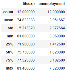
ii. Visualize the Data
Use the histPlotAll() function from functions.py to plot a histogram for each numeric feature:
# View univariate histgram plots
histPlotAll(dataset)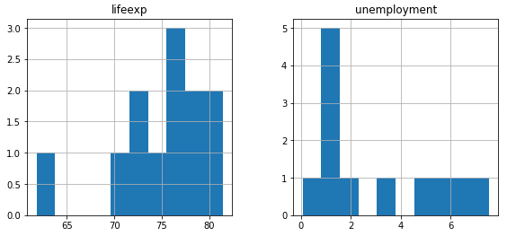
Use the boxPlotAll() function from functions.py to plot a box plot for each numeric feature:
# View univariate box plots
boxPlotAll(dataset)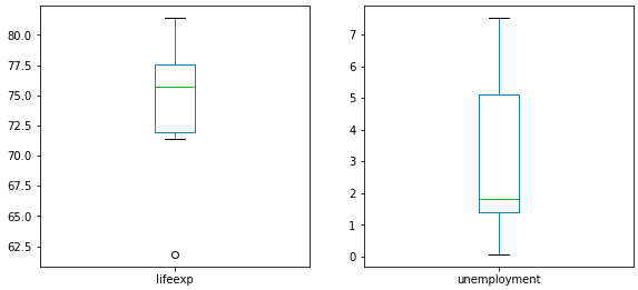
And the classComparePlot() function from functions.py to plot a comparative histogram for the two classes:
# View class split
classComparePlot(dataset[["happiness","lifeexp","unemployment"]], 'happiness', plotType='hist')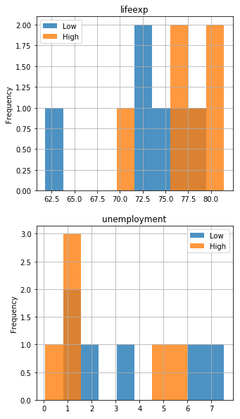
4. Prepare the Data for Supervised Machine Learning
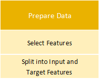
i. Select Features and Split Into Input and Target Features
We can select happiness as the feature to predict ( ) and lifeexp and unemployment as the features to make the prediction ( ):
# Split into input and output features
y = dataset["happiness"]
X = dataset[["lifeexp","unemployment"]]
X.head()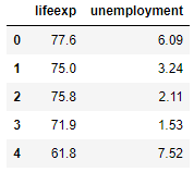
y.head()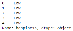
5. Build a Model
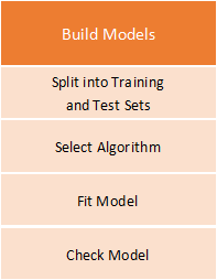
i. Split Into Training and Test Sets
Use the train_test_split() function in sklearn to split the sample set into a training set, which we will use to train the model, and a test set, to evaluate the model:
# Split into test and training sets
test_size = 0.33
seed = 7
X_train, X_test, y_train, y_test =  train_test_split(X, y, test_size=test_size, random_state=seed)
Note that I have requested ⅓ of the data be held back as the test set. I have also set the random_state parameter to a seed of seven. This requests a random sampling of the data but ensures we can always get the same random sampling if we rerun the experiment. When we tweak the model, it ensures that any changes are due to the tweaking, and not to the random sampling being different. You can change the random sample by changing the seed to another integer value.
Let's look at the four samples produced and confirm the randomness of the selection:
X_train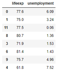
X_test
y_train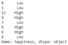
y_test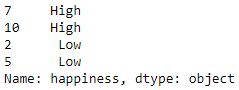
ii. Select an Algorithm
Create a model using the sklearn decision tree algorithm:
# Select algorithm
model = DecisionTreeClassifier()
iii. Fit the Model to the Data
Now take the training set and use it to fit the model (i.e., train the model):
# Fit model to the data
model.fit(X_train, y_train)
iv. Check the Model
Next, assess how well the model predicts happiness using the training data, by “pouring” training set X into the decision tree:
# Check model performance on training data
predictions = model.predict(X_train)
print(accuracy_score(y_train, predictions))
1.0
The model has performed really well - 100%!
6. Evaluate the Model
i. Compute Accuracy Score
Let’s pour test set into the decision tree and see what it predicts:
# Evaluate the model on the test data
predictions = model.predict(X_test)
Look at the predictions it has made:
predictionsarray(['Low', 'High', 'High', 'Low'], dtype=object)
And compute the accuracy score:
print(accuracy_score(y_test, predictions))0.5
We can show the model predictions with the original data, with the actual happiness value:
df = X_test.copy()
df['Actual'] = y_test
df['Prediction'] = predictions
df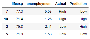
What Rules Did Sklearn Come Up With?
At this point, the model produced by sklearn is a bit of a black box. There is no set of rules to examine, but it is possible to inspect the model and visualize the rules.
For this code to work, you need to first install Graphviz by running the following from a terminal session:
conda install python-graphviz
You can then run the following code, which uses a function from functions.py:
viewDecisionTree(model, X.columns)And see the decision tree rules:
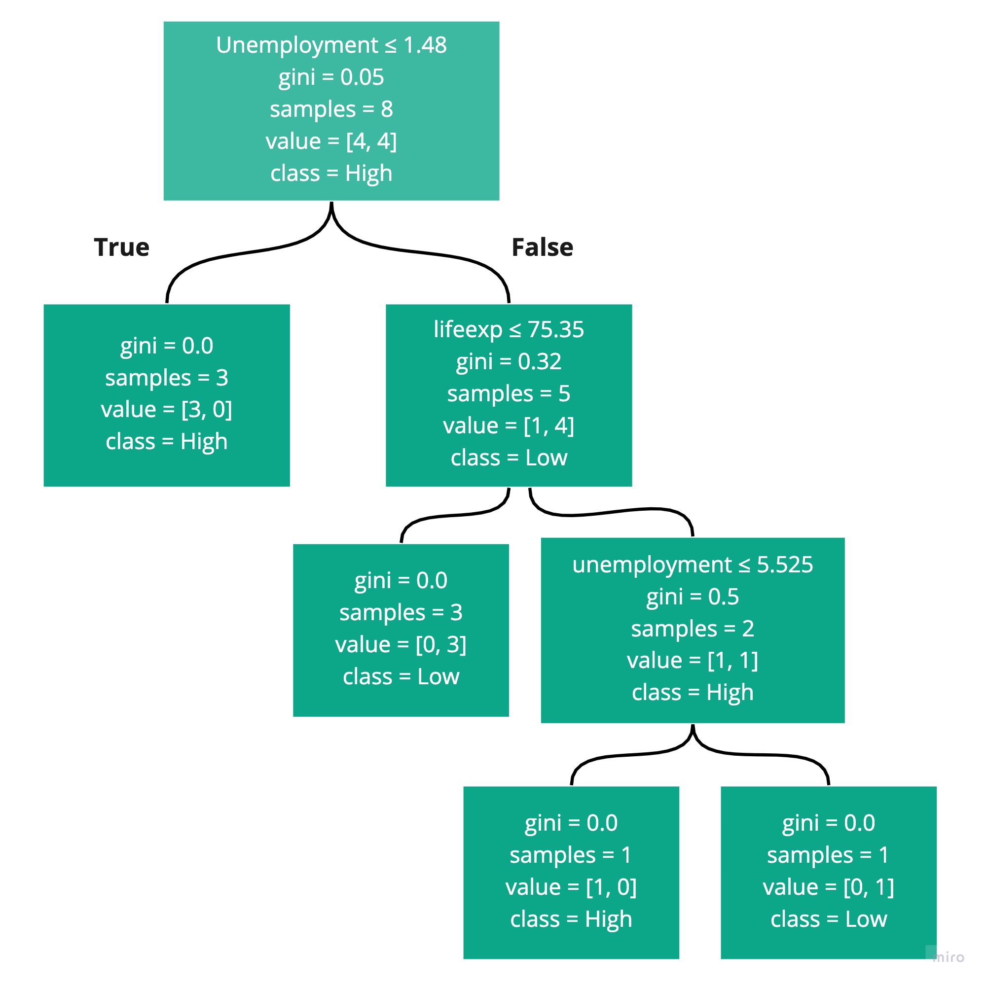
You can see that the first rule is to check if unemployment is below or equal to 1.48 , and if so, classify the sample point as high. The next rule checks if lifeexp is below or equal to 75.35, and if, so classify the sample point as low. The third and final rule checks if unemployment is below or equal to 5.525, and if so, classify it as high. Any other sample points get classified as low.
There are probably a couple of questions in your mind:
What is Gini?
How did sklearn come up with the rules and specifically the boundary values like 5.525?
We will examine the construction of decision trees and answer these questions in the next chapter.
Recap
You built your first machine learning model! It’s not a great one, mainly because the dataset was so small. You’ve learned the process for building such models, and how a simple algorithm - decision tree - can be used to perform a classification task.
In the next part, we will build something more solid by exploring some other techniques. But for now, it's time to test your knowledge!
