Table of contents
- Part 1
Identify Common Machine Learning Problems
- Part 2
Evaluate the Performance of a Machine Learning Model
- Part 3
Improve the Performance of a Machine Learning Model
Table of contents
- Part 1
Identify Common Machine Learning Problems
- Part 2
Evaluate the Performance of a Machine Learning Model
- Part 3
Improve the Performance of a Machine Learning Model
Identify the Problems of Overfitting and Underfitting
Welcome to this course on evaluating and improving machine learning models!
In the previous course, Train a Supervised Machine Learning Model, we saw how to take an algorithm, build a model and fit the model with some data. The model represented the relationships between the input features and the target feature, and we used that model to predict the target feature from the input features.
We saw that when we fitted different models with the same data we got different results, with some models performing better than others. We also saw that some models performed really well on the training data, but poorly on the test data. Other models performed quite consistently.
In this course, we will look at how to achieve this challenging goal. We will examine:
Some of the problems exhibited by models
Better ways to evaluate how effective our models are
Better ways to decide what input features to use for our models
Ways to improve the performance of your models
In this first chapter, we will look at some of the reasons why models may perform poorly or inconsistently. We use the terms underfitting and overfitting to describe this poor or inconsistent performance. Don't worry, by the end of this chapter, you will have a good understanding of what these terms mean. ;)
First of all, we need to understand the idea of the bias-variance tradeoff, which is a fundamental characteristic of all supervised learning models.
Understand the Bias-Variance Tradeoff
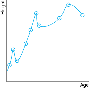
Take a look at this chart, which plots the age and heights of a group of children.
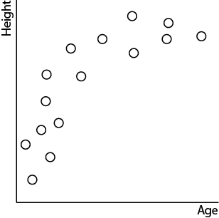
As you can see, children tend to grow quite rapidly in their early years, but that growth slows in their late teen years.
When we create a model to represent this relationship, our aim is to draw some sort of line through the points and to use that line to predict height from age. This is a typical regression problem. The better the line represents the data, the better our model will be.
To fit the model, we would select a subset of the data, say two-thirds, and use it as training data. The remaining data we will use as test data to test our model.
We may use linear regression to find a line of best fit through the training data. In this case, our model may look something like this:
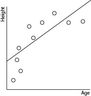
It's a simple model. But is it too simple? Does it capture the relationship well? Does it capture the slowing growth in the teen years?
Instead of using linear regression, we may find another algorithm, let's call it squiggle regression (it's not a real algorithm >_<), that fits the following line through the data:
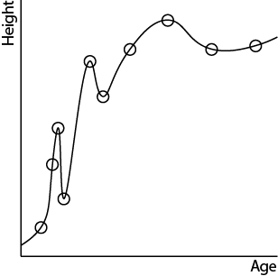
It's a much more complex model. It captures all the twists and turns of the data, fitting the training data perfectly. But again, does it capture the relationship well? Does it capture the general trend?
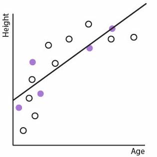
Let's put our test data back on the chart and see how each model performs. First the linear regression model, with the test data showing as purple dots:
Now the squiggle regression model:
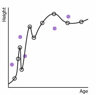
How does our perfect squiggle model look now? Not so good!
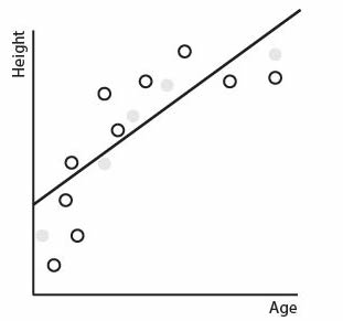
If we take a completely new data set, one not used for training or testing, we can see that the performance of the linear regression model is quite consistent with the training and test runs:
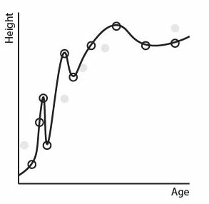
The performance of the squiggle regression model again doesn't match its training set performance:
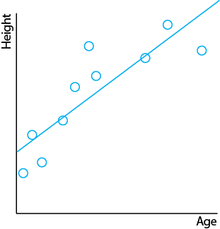
What if we retrain the model with a different random training set? Here, the blue circles represent totally new observations of children's ages and height. First linear regression:
Now squiggle regression:
The differences in the two models created with each of the two algorithms can be seen more clearly if we overlay them:
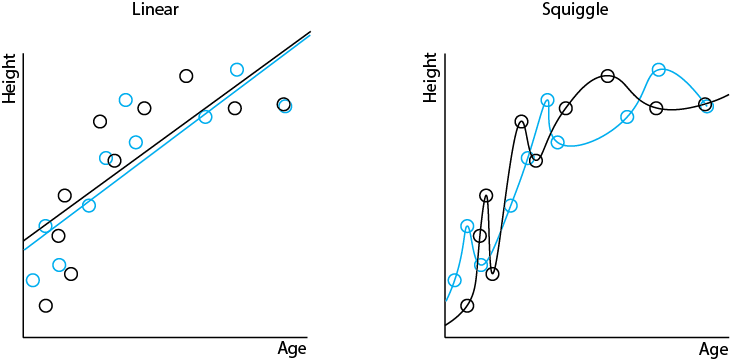
What do you notice?
With linear regression, we get a very similar result with the two models. Both linear regression models will make similar predictions on the same input data. With squiggle regression, we get very different results between the two models. The two squiggle regression models can make very different predictions of height with the same age input. The following diagrams show this difference:
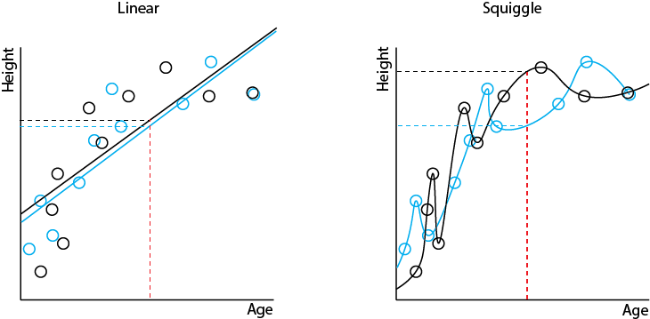
Linear regression hasn't managed to capture the true relationship between age and height. It has over-simplified it. Indeed, it misses the fact that children grow rapidly in their early years and then much more slowly in their late teenage years. It's biased towards the average height. We say it has high bias. On the other hand, it does perform consistently. If we build models with different training data, we will get a reasonably consistent model, making reasonably consistent predictions. We therefore says that it has low variance.
Squiggle regression has managed to capture the difference in growth speed in early years and late teen years. We say it has low bias. On the other hand, it is quite inconsistent, coming up with different relationships, and therefore different predictions, with different training data. We therefore say it has high variance.
There is a classic bulls-eye diagram by Scott Fortmann-Roe that you will see in many discussions on bias and variance. Each dot on the target is the result of an individual model. Each model is trained on different data.
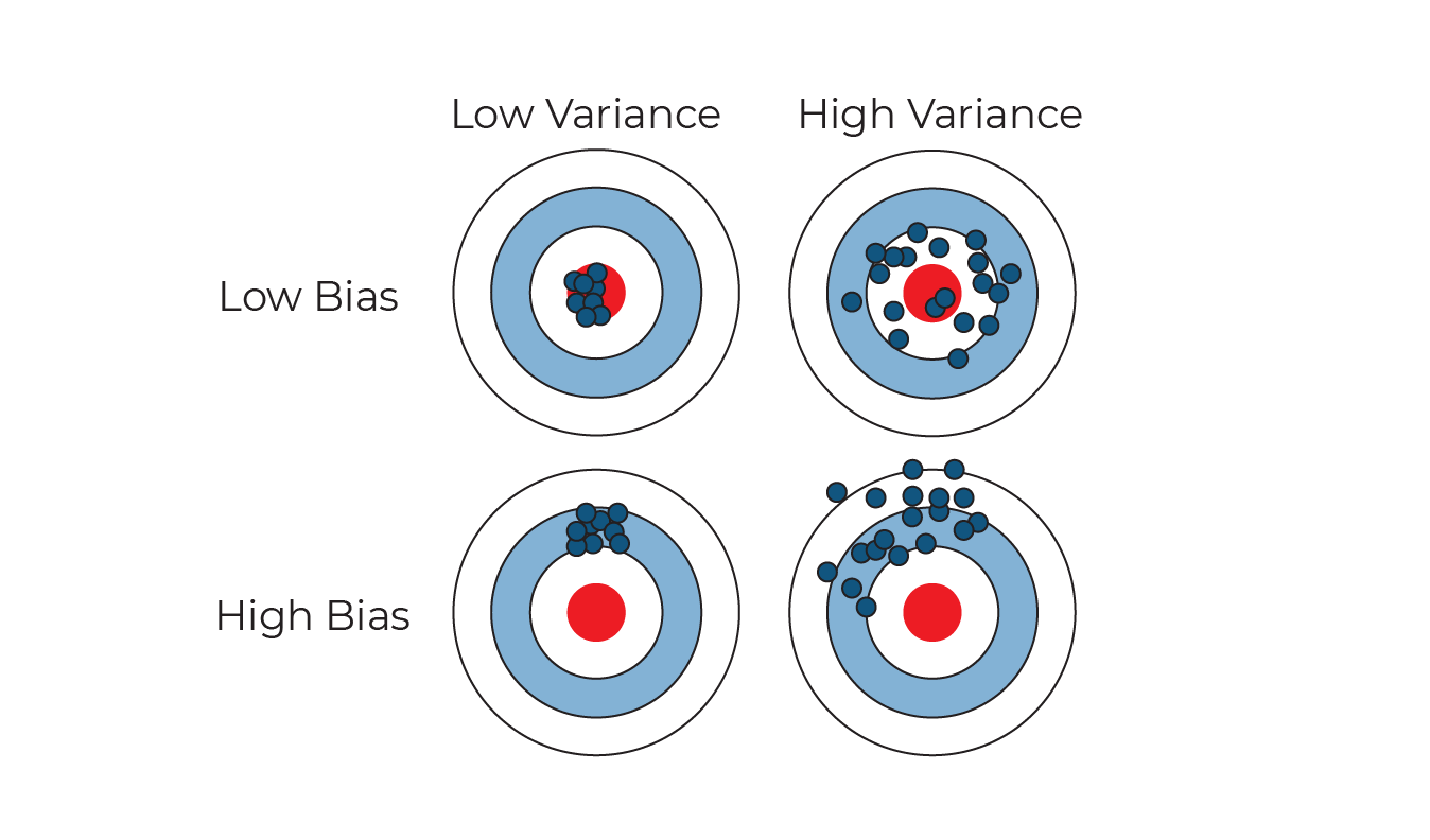
A hit close to the bulls-eye means a good model, that makes good accurate predictions.
A hit away from the bulls-eye means a model that performs less well, maybe being susceptible to outliers in the data.
Understand Underfitting and Overfitting
In data science, we use the terms underfitting and overfitting to describe methods that lead to models that sit outside of a good bias/variance tradeoff.
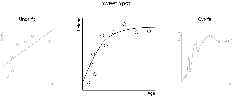
In the above example, our linear regression model is underfit. It is too simple and doesn't capture the complexities in the relationship between age and height.
But our squiggle regression model is overfit. It is too complex and has a very fixed and specific idea of the underlying relationship based on the training data. It isn't very flexible when presented with new data.
Building machine learning models is a constant battle to find the sweet spot between underfitting and overfitting.
Recognizing Underfitting and Overfitting
How can you tell if your model is suffering from underfitting or overfitting?
A model that performs much better on training data than on the test data is likely to be overfit. So for example, if we had 95% accuracy on the training data, but only 60% accuracy on the test data it would be a good indicator of an overfit model.
A model that performs poorly is a sign that you may have an underfit model. But note that this could also be a sign that you have a poor feature set or the relationships in the data are inherently poor.
Avoiding Overfitting
Here are some ways to avoid overfitting when building your models. We will take a deep dive into these concepts later in the course.
Hold back a test set
Always hold back a test set, training your model with around 2/3 or 3/4 of the data and using the rest for testing the resulting model. This is the approach we used in the previous course, Train a Supervised Machine Learning Model. Use the test set to prove that your model performs well on unseen data. If it doesn't, go back and improve your model.
Resampling with Cross-validation
This approach generates multiple train-test splits and fits the model with each split in turn. We can check to ensure we get consistently good results from each split. Use cross-validation to prove that your model performs well on different cuts of unseen data. If it doesn't, go back and improve your model.
Feature selection
Overfitting can sometimes result from having too many features. In general, it is better to use a few really good features rather than lots of features. Remove excessive features that contribute little to your model.
Regularization
This approach is used to "tune down" a model to a simpler version of itself. Apply regularization to reduce a model's tendency to overfit.
Summary
Bias is the tendency of models to provide inaccurate predictions.
Variance is the tendency of models to provide very different results when trained with different cuts of data.
There is always a trade-off between bias and variance
Underfitting occurs when our model is too simple to capture the complexities of the relationships in the data. A model that consistently performs poorly may be underfit.
Overfitting occurs when our model is too complex to capture the underlying relationships in the data. A model that performs well on training data, but poorly on test data is overfit.
In the next chapter, we will be exploring a common machine learning problem called multicollinearity. Ready? Let's go!
Ever considered an OpenClassrooms diploma?
- Up to 100% of your training program funded
- Flexible start date
- Career-focused projects
- Individual mentoring
Find the training program and funding option that suits you best
