Work With Large Quantities of Data

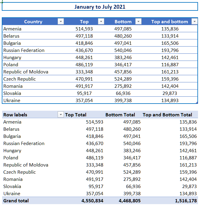
In this download file, you’ll find a table and a matching Pivot Table.
Insert Calculated Fields
You have just found out that the table sales figures need to be reduced, as a 5% tax will be applied.
You can do this calculation within your Pivot table, using calculated fields:
Select one cell in the Pivot Table.
Go to “PivotTable Analyze” and then “Calculations”, and click on the
 icon.
icon.Click on the “Calculated Field...” row. The calculated field setup window opens:
In the calculated field name, enter “Top minus tax.”
Complete the Formula field by double-clicking on the “Top” field and adding “*0.95” to remove the 5% tax.
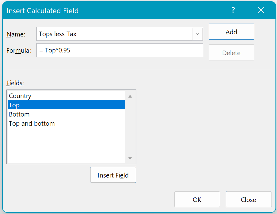
Click OK, and Excel automatically adds the field to your Pivot Table.
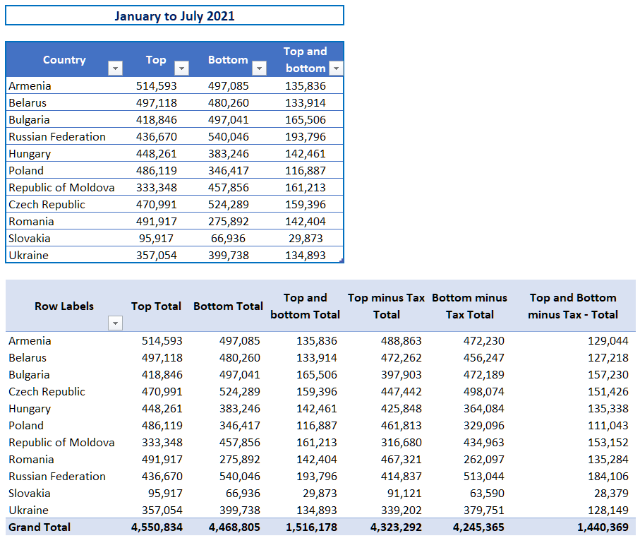
Repeat the same process to create calculated fields for “Bottom minus tax” and “Top and bottom minus tax.”
The Pivot Table now contains six columns of data:
All you need to do now is to remove the three original columns from the Pivot Table:
Select one cell from the first heading, “Top Total.”
Right-click to open the context menu, then click on the
 row.
row.Do the same for “Bottom Total” and “Top and Bottom Total.”
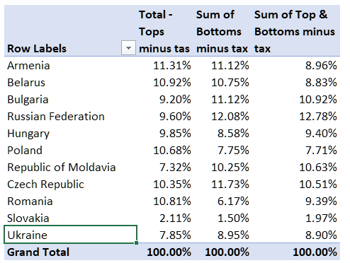
And you’re left with the result! 😊
Do Calculations on Existing Fields
You want to get the weighting of each country for each category.
There is a really quick way of doing this calculation:
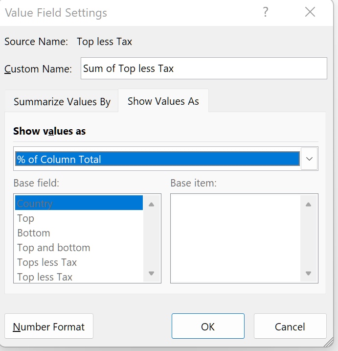
Select the header cell for the first calculated column.
Open the context menu and select the
 command.
The default Excel calculation is a sum. Go to the “Show Values As” tab to select another calculation. In this case, we have selected “% of Column Total.”
Do the same for the other two calculated fields, “% of Bottom minus tax” and “% of Top and bottom minus tax.”
You should get the following result:
Use Power Pivot to do More
If you work with multiple data sources and databases containing large quantities of data on a daily basis, you might want to consider Excel’s Power Pivot add-in.
This tool helps you to create complex data models, which are more tailored than the adjustments you can make using Excel’s basic features.
Over to You!
Download this file and do the following:
“P4C3-TCD” tab: in the Pivot Table on the right, add a calculated column called “Country share,” which sets out the share for each country (the total at the bottom will be 100%).
Answer Key
You can find the answer key here and watch the video below to check your work.
Let’s Recap!
Quickly analyze your data using Pivot Table calculated fields.
You’re now done with creating and analyzing your dashboard. 🥳 Join me in the next chapter to find out how to set up automatic updates for your dashboard!
