Initiez-vous au Deep Learning

Dans ce chapitre, nous allons découvrir les principes d’un modèle génératif et apprendre à construire de tels modèles en réseaux de neurones.

  $$\(\newcommand{\abbva}{\texttt{v.a.}} \newcommand{\abbea}{\texttt{e.a.}} \newcommand{\abbddp}{\texttt{d.d.p.}} \newcommand{\vaX}{\mathrm{X}} \newcommand{\vaY}{\mathrm{Y}} \newcommand{\msR}{\mathbb{R}} \newcommand{\sH}{\mathcal{H}} \newcommand{\sV}{\mathcal{V}} \newcommand{\sW}{\mathcal{W}} \newcommand{\sX}{\mathcal{X}} \newcommand{\sY}{\mathcal{Y}} \newcommand{\sZ}{\mathcal{Z}} \newcommand{\va}{\mathbf{a}} \newcommand{\vb}{\mathbf{b}} \newcommand{\ve}{\mathbf{e}} \newcommand{\vf}{\mathbf{f}} \newcommand{\vg}{\mathbf{g}} \newcommand{\vh}{\mathbf{h}} \newcommand{\vm}{\mathbf{m}} \newcommand{\vq}{\mathbf{q}} \newcommand{\vr}{\mathbf{r}} \newcommand{\vu}{\mathbf{u}} \newcommand{\vv}{\mathbf{v}} \newcommand{\vw}{\mathbf{w}} \newcommand{\vx}{\mathbf{x}} \newcommand{\vy}{\mathbf{y}} \newcommand{\vz}{\mathbf{z}} \newcommand{\valpha}{\boldsymbol{\alpha}} \newcommand{\vze}{{\Pi}} \newcommand{\mA}{\mathbf{A}} \newcommand{\mB}{\mathbf{B}} \newcommand{\mC}{\mathbf{C}} \newcommand{\mF}{\mathbf{F}} \newcommand{\mG}{\mathbf{G}} \newcommand{\mH}{\mathbf{H}} \newcommand{\mQ}{\mathbf{Q}} \newcommand{\mR}{\mathbf{R}} \newcommand{\mP}{\mathbf{P}} \newcommand{\mS}{\mathbf{S}} \newcommand{\mK}{\mathbf{K}} \newcommand{\norml}{\mathcal{N}} \newcommand{\normc}{\boldsymbol{\mu}} \newcommand{\norms}{\boldsymbol{\Sigma}} \newcommand{\normf}{f_{\mathcal{N}}} \newcommand{\dyncolor}[1]{ {\color{magenta!50!black} #1 }} \newcommand{\obscolor}[1]{ {\color{yellow!50!black} #1 } } \newcommand{\priorcolor}[1]{ {\color{blue!50!black} #1 } } \DeclareMathOperator*{\argmax}{arg\,max} \DeclareMathOperator*{\mmax}{max} \DeclareMathOperator*{\argmin}{arg\,min} \DeclareMathOperator*{\mmin}{min} \DeclareMathOperator*{\msup}{sup} \DeclareMathOperator*{\minf}{inf} \)$$ 

Qu’est-ce qu’un modèle profond génératif (sans vraisemblance) ?

Likelihood-free Deep Generative Model

C'est un modèle génératif qui permet d'apprendre une distribution approchée $\$\backslash (Q\backslash )\$$ d'un ensemble de points $\$\backslash (p\; \backslash sim\; P\backslash )\$$, une distribution inconnue. On peut tirer un échantillon de $\$\backslash (Q\backslash )\$$ , mais on ne pourra pas calculer la vraisemblance d'un échantillon par rapport à la distribution modélisée.

Décodeur d'un autoencoder (AE) comme modèle générateur

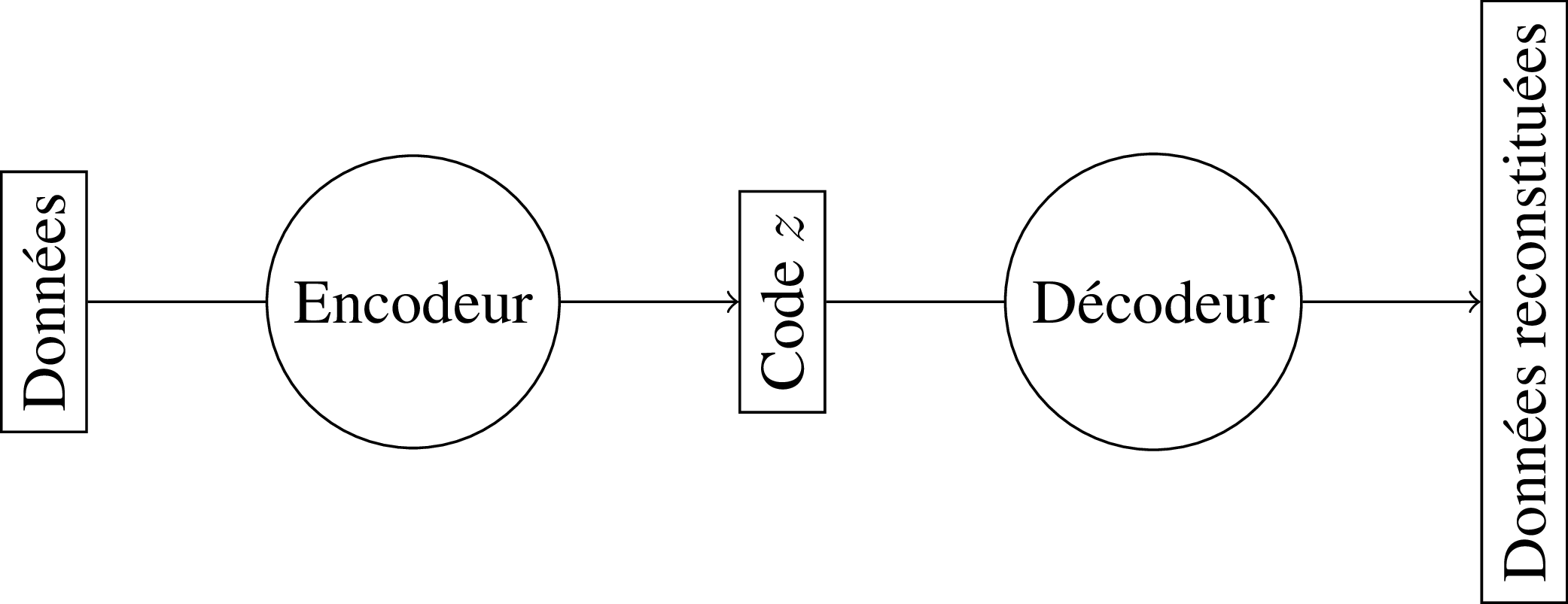
Pour ce faire, on peut essayer un autoencodeur (les réseaux diabolos). On apprend un AE profond sur une base d'images :

Puis on garde juste la partie décodeur :

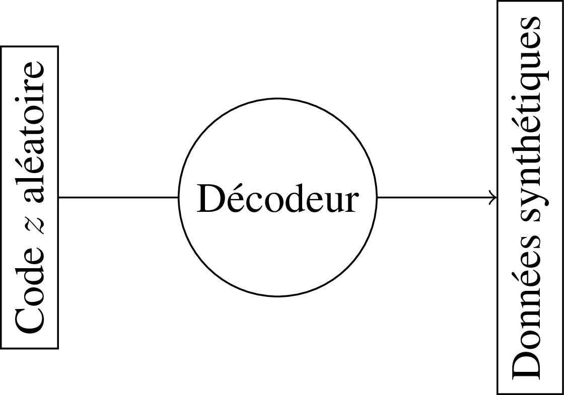
On tire un code $\$\backslash (z\backslash )\$$ au hasard, et on le passe dans le décodeur pour générer une donnée synthétique.

Le problème, c'est qu'on ne connaît pas la distribution du code, et il est fort probable que l'on tombe sur une image qui n'est pas réaliste. Pour cela, on peut forcer la distribution de la représentation réduite lors de l'apprentissage ; c'est ce qu'on appelle des VAE, pour Variational Auto-Encoder.

Apprentissage adverse, ou Generative Adversarial Network (GAN)

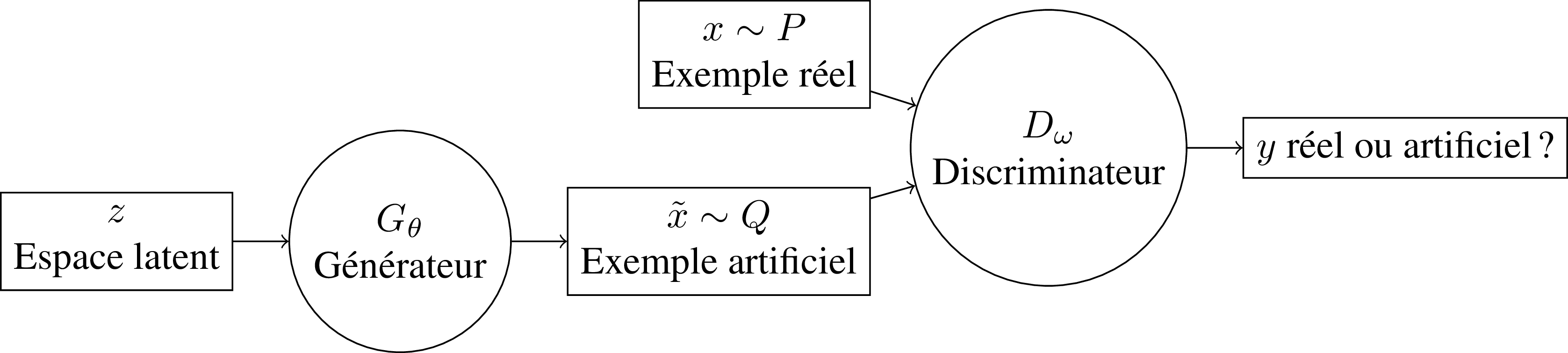
Une autre technique de construction des modèles génératifs se base sur deux réseaux profonds :

• un générateur ;

• un discriminateur.

Le générateur crée un exemple synthétique à partir d'un code tiré d'une distribution aléatoire connue.

Le discriminateur, lui, essaie de déterminer si l'exemple qu'il voit à son entrée est un exemple réel ou un exemple synthétique.

Les deux réseaux sont regroupés en un seul réseau appelé Generative Adversarial Network (GAN).

Lors de l'apprentissage, les deux réseaux sont en positions adverses :

• le discriminateur essaie de déterminer au mieux la provenance des exemples (e.g., réel ou artificiel ?) ;

• le générateur essaye de tromper le discriminateur.

Objectif d'un GAN

La fonction objectif d'un GAN s'écrit de la façon suivante :

\begin{eqnarray*}
V(\omega,\theta)&=&-\frac{1}{2}\mathbb{E}_{x\sim P}log(D_{\omega}(x))-\frac{1}{2}\mathbb{E}_{z\sim Z }log(1-D_{\omega}(G_{\theta}(z)))\\
&=&-\frac{1}{2}\mathbb{E}_{x\sim P}log(D_{\omega}(x))-\frac{1}{2}\mathbb{E}_{\tilde{x}\sim Q_{\theta} }log(1-D_{\omega}(\tilde{x}))\\
\end{eqnarray*}

Le discriminateur minimise $\$\backslash (V(\backslash omega,\backslash theta)\backslash )\$$ sur $\$\backslash (\backslash omega\backslash )\$$ à $\$\backslash (\backslash theta\backslash )\$$ fixé.

Le générateur maximise $\$\backslash (V(\backslash omega,\backslash theta)\backslash )\$$ sur $\$\backslash (\backslash theta\backslash )\$$ à $\$\backslash (\backslash omega\backslash )\$$ fixé.

On cherche donc un point col, un équilibre de Nash.

Pour des questions numériques (problème de gradient), un objectif différent est utilisé en pratique, mais il ne présente pas les mêmes propriétés de stabilité.

Exemples d'utilisation

Voici un article qui propose un exemple de GAN appris sur des photos de chiens, cf. la figure 3 de l'article suivant : Denton, Emily L., Soumith Chintala, and Rob Fergus. "Deep generative image models using a laplacian pyramid of adversarial networks."Advances in neural information processing systems. 2015.

Un exemple similaire, mais sur des visages humains, se trouve aux liens suivants :

Article explicatif

Code en Torch7

Exemple GAN autoencoder

On peut aussi construire une architecture combinée entre GAN et AE :

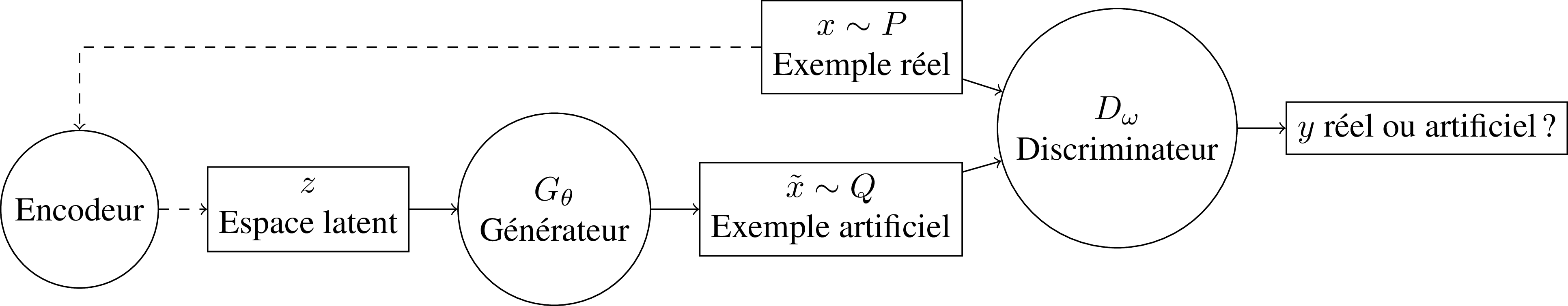
Le générateur est utilisé comme décodeur d'un AE. L'encodeur ainsi appris permet de passer de l'espace de grande dimension à l'espace latent.

Cela permet des manipulations dans cet espace latent. Un homme avec des lunettes moins un homme plus une femme donne une femme avec des lunettes, cf. la figure 7 de l'article suivant : Radford, A., Metz, L., Chintala, S. (2015). Unsupervised representation learning with deep convolutional generative adversarial networks. arXiv preprint arXiv:1511.06434.

On peut, avec ce système, produire par exemple du morphing : Karras, T., Aila, T., Laine, S., & Lehtinen, J. (2017). Progressive growing of gans for improved quality, stability, and variation. arXiv preprint arXiv:1710.10196.

Voici un exemple en vidéo.

Tout l'univers des GAN

De nombreuses applications sont possibles avec le GAN :

• colorisation d'images en noir et blanc ;

• segmentation/cartographie ;

• à l'inverse, générer une image synthétique à partir d'une carte ;

• inpainting ;

• prédiction de trames vidéo.

Pour les découvrir, regarder les articles dans la section Pour aller plus loin.

Allez plus loin

Goodfellow, I., Pouget-Abadie, J., Mirza, M., Xu, B., Warde-Farley, D., Ozair, S., Bengio, Y. (2014). Generative adversarial nets. In Advances in neural information processing systems (pp. 2672-2680)

Goodfellow, I. (2016). NIPS 2016 Tutorial: Generative Adversarial Networks. arXiv preprint arXiv:1701.00160

Makhzani, A., Shlens, J., Jaitly, N., Goodfellow, I., Frey, B. (2015). Adversarial autoencoders. arXiv preprint arXiv:1511.05644.

En résumé

Ce chapitre introduit la notion d'apprentissage adverse. C'est un type d'apprentissage qui permet de synthétiser des exemples artificiels de données à partir d'exemple réels. Il est très performant sur la modalité image. En association avec un autoencodeur, il permet des manipulations sur l'espace latent des données, comme le morphing ou l'inpainting.