Discover the Principles of Multivariate Exploratory Data Analysis
Hello! Welcome to the course on multivariate exploratory data analysis!
I am looking forward to guiding you through the vast world of statistics. ^^ If you have not already, I invite you to check out the previous course, Perform an Initial Data Analysis. In that course, we dealt with descriptive statistics. Just as the name suggests, the purpose of descriptive statistics is to describe either:
a single variable
or the relationship between two variables.
So where do we stand in this course?
Well, in this course, we are going to go one step further and study the relationship between 3 or more variables at the same time. This is called multivariate exploratory analysis.
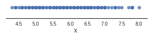
On a paper or on a screen, it is easy to make a graph with 2 dimensions. It would have 2 axes: one horizontal and one vertical, as shown in the scatterplot above.
In 3 dimensions, depth is added. Here, we can still manage to visualize our data - just imagine a room full of ping pong balls. But what happens when we move to 4 dimensions? It comes very hard for the human brain to imagine. Fortunately, in statistics, we have techniques that work with a large number of dimensions. These techniques can also be used to reduce the number of dimensions to something that works better on a human scale. In this course, we are going to be looking at these techniques.
What are the Advantages of Multivariate Analysis?
The answer is simple: you can extract a lot more information from your data when you study the relationship between multiple variables than when you study variables separately (one by one).
Let's take a look at an example:
Imagine asking customers to rate their satisfaction level through five criteria, on a scale of one to five, with one being "not at all satisfied" and five being "very satisfied". Here are the five criteria:
Quality of the products
Price of the products
Quality of the overall service
Smoothness of the purchase process
Friendliness of the staff
Imagine that 8 customers answered. You will end up with a table that looks like this:
| Product Quality | Price | Service Quality | Smoothness | Friendliness |
Customer 1 | 3 | 3 | 3 | 5 | 5 |
Customer 2 | 2 | 3 | 2 | 5 | 4 |
Customer 3 | 2 | 3 | 3 | 4 | 5 |
Customer 4 | 1 | 1 | 1 | 1 | 1 |
Customer 5 | 5 | 5 | 4 | 3 | 3 |
Customer 6 | 4 | 5 | 5 | 2 | 3 |
Customer 7 | 5 | 5 | 5 | 3 | 3 |
Customer 8 | 1 | 1 | 1 | 1 | 1 |
mean | 2.875 | 3.25 | 3 | 3 | 3.125 |
If you look at the mean for each criterion, you're performing a univariate analysis, because you're looking at each variable (each column) one by one. This leads us to think that customers have an overall satisfaction level that is around three, whatever the criterion may be.
But what we are interested in here, is the customer profile, that is, the whole of their five answers. Here, a customer is a five-value "package" (the term five-dimensional vector is preferred). As it is the customer profile that interests us, we cannot just look at each variable separately, the five-dimensional vector characterizing each customer must be looked at.
We can see for example that two customers answered "1" in all criteria (individuals 4 and 8). This is a classic phenomenon: every time a satisfaction survey is submitted, some people who wish to express their dissatisfaction answer "very dissatisfied" (or the opposite) for each question without even really reading the question.
Besides the "hyper-critics", there are two quite distinct groups of people: those who are very satisfied with the purchase process, but only averagely so with the price (individuals 1, 2, and 3), and conversely, those who are very satisfied with the price, but only moderately so with the purchase process (individuals 5, 6, and 7).
What are the Different Multivariate Analysis Techniques?
If your sample is represented by a table with 100,000 rows and 1,000 columns, it can be a bit tricky to analyze! The sheer size of the data set will make it difficult to identify patterns. Furthermore, some statistical treatments performed by computers can take a very long time (sometimes several days, several months, or more!).
This course focusses on 2 methods to simplify the data in order to make analysis easier:
Dimensionality reduction
Clustering
For each of these methods, there are various algorithms we can apply. In this course we will focus on a few key ones:
Dimensionality reduction using Principal Component Analysis
Clustering using K-means and Hierarchical clustering
Principal Component Analysis (PCA)
Principal Component Analysis (PCA) lets you reduce the number of variables by finding new variables that combine the essence of several others. Finding such variables allows us to replace several columns in a table with just a few. In so doing, we will lose a little information, but we can make an informed choice by weighing up the benefit of simplifying the data against the downside of the lost information.
Clustering
As for clustering, it allows you to group similar individuals, that is to say, it will partition the entire set of individuals into groups. Grouping individuals, here, is synonymous with grouping rows in a table of data. Sometimes, you can group 100,000 rows into three groups that are homogeneous enough that you only need to examine the general profile of each group, so only three rows!
Clustering has multiple applications. For example, it is widely used in marketing to segment a client database. By forming "groups" of customers and studying their characteristics (in terms of age, of centers of interest, etc.), marketers can make their marketing campaigns more targeted.
Another example is picture analysis: when two pixels of a photograph are very similar in terms of color, they can be grouped into just one color. Thus, the number of colors on a picture is reduced optimally, and therefore its size is also reduced (here is an example using sklearn).
The Concept of Euclidean Space
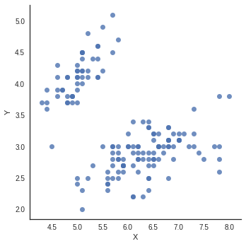
Let's have a look at a scatter plot from earlier:

Here, individuals are represented by points, each of which have two coordinates: a horizontal axis and a vertical axis. We say that the data is shown in a two-dimensional space, because in order to place the points, two variables describing the individuals were selected. To some extent, we associate the notion of a variable with that of a dimension.
We call the space in which we plot these points a Euclidean space. In the scatter plot above, the points are drawn in a two-dimensional Euclidean space.
The notion of distance
If I asked you for the distance between two points A and B on a two-dimensional graph such as the one below, how will you proceed?
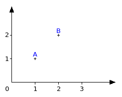
Some of you will have used a graduated ruler to measure, others will have been more daring and will have calculated the distance using the coordinates of both points. In either case though, you will have reached the same result (here, √2, or roughly 1.41).
What you measured instinctively is called Euclidean distance. It's the measurement of the shortest distance between A and B. There are other ways of measuring distance, but we won't concern ourselves with those in this course.
Point clouds
When we represent the individuals from a sample with points in Euclidean space or 3 or more dimensions, the whole of those points is called a point cloud. Poetic, isn't it? Like those summer afternoons spent lying on the grass, looking up at the clouds in the sky. I'm sure you've already played that game: trying to compare the shapes of clouds to animals, or other known objects.
When it comes to statistics, we do the same thing, we describe point clouds: what shape are they? Are they spread out, narrow, dense, big, small? What is their position?
A cloud that's spread out within the space will, for instance, represent individuals that are very different from each other. Maybe the cloud will contain agglomerations, that is to say, denser zones. In this case, it means that there are groups of similar individuals, who are different from the other groups.
Just as with our two-dimensional space, we can measure the distance between points in 3 or more dimensions.
Variance in Euclidean Spaces
In the previous course, we encountered the concept of empirical variance as a measure of dispersion, or how much our data is spread out. We saw how this could be calculated for a single variable. Calculating the variance involved measuring the distance from each point to the mean. The mean is our central point, the "centre of gravity" of our data.
Moving up to 2, 3 or more dimensions, we can still calculate a mean point, the centre of gravity of all our data points. And we can still measure the distance from all our data points to the centre of gravity. And thus we can still calculate the variance of the point cloud.
Supervised or unsupervised?
In machine learning, a distinction is made between supervised and unsupervised treatments.
The unsupervised approach consists in exploring data without a guide, whereas the supervised approach learns from examples in order to make predictions.
The techniques of Principal Component Analysis and clustering that we will look at in this course are unsupervised tasks. There is no guide. The algorithms will discover patterns in the data without knowing them in advance.
The picture below puts these different techniques into context: 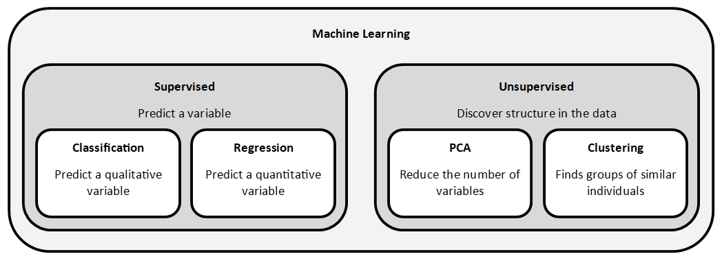
Recap
Multivariate exploratory analysis is the study of 3 or more variables. It is used to examine a profile, or in other words, a set of characteristics.
"Number of variables" is the same as saying "number of dimensions".
Dimensionality reduction and clustering are two techniques that are used to reduce the number of dimensions in a dataset.
The space in which we plot points is called the Euclidean space.
The shortest distance between 2 points is called the Euclidean distance.
A point cloud is a set of data points in Euclidean space.
Variance in Euclidean space is a measure of dispersion (how much the data is spread out).
