Perform an Initial Data Analysis

There is more to life than histograms!

It is also possible to present variables in the form of a table. It’s not as pretty, of course, but in some cases, this representation is better suited, or supplements, a graphic representation. We will look at four cases, corresponding to the four variable types.

Let's Start With Some Vocabulary

So that the two of us can communicate, you and I, we need to adopt a common language. So we are going to name the different objects we will be manipulating in this chapter.

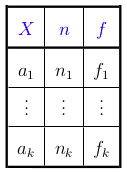
Here we are working with the bank statement sample, which is made up of transactions. Note that  $\$\backslash (n\backslash )\$$ will represent the number of banking transactions: this is our sample size.

Next, the variable we will be analyzing will be referred to as $\$\backslash (X\backslash )\$$ .

 $\$\backslash (X\backslash )\$$  is not particularly concrete: it’s just a variable. For example, amount is a variable.

Our data set contains a number of different values for the amount variable: 1.43, 80, 2.20, etc. No more theory now - all practice! We’ve got real values in front of us. The number of values in our sample is $\$\backslash (n\backslash )\$$ . So we can express these values as ( $\$\backslash (x1,...,xn\backslash )\$$).

When referring to variables, it’s best to use a capital letter. However, when referring to observations of the variable, lower case letters are used. Here, ( $\$\backslash (x1,...,xn\backslash )\$$) is an observed realization of the random variable $\$\backslash (X\backslash )\$$.

Discrete Quantitative and Qualitative Variables

If $\$\backslash (X\backslash )\$$ is qualitative (or even discrete quantitative), it can take a number of categories. For example, categ can take the categories “GROCERIES,” “RENT,” “TRANSPORTATION,” etc. We will refer to these categories as {$\$\backslash (a1,...,ak\backslash )\$$}, where $\$\backslash (k\backslash )\$$ indicates the number of categories.

Continuous Quantitative Variables

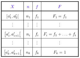
To present continuous quantitative variables, we will group the values of variable X into bins, which will be k in number. These bins will be expressed as follows:

  $\$\backslash (\backslash \{[a\_1\text{'},a\_2\text{'}[,...,[a\_k\text{'},a\_\{k+1\}\text{'}[\backslash \}\backslash )\$$

Representing Variables in the Form of a Table

Qualitative Variables

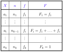
For qualitative variables, simply count the number of values for each category. This number is referred to as the occurrence of the category.

So, for a category $\$\backslash (ai\backslash )\$$ (where $\$\backslash (i\backslash )\$$ is between $\$\backslash (1\backslash )\$$ and $\$\backslash (k\backslash )\$$ of course!), the occurrence is expressed as $\$\backslash (n\; I\backslash )\$$. If we add up the occurrences of all of the categories, we get $\$\backslash (n\backslash )\$$: the sample size.

If we divide the number of occurrences by $\$\backslash (n\backslash )\$$, we get the frequency, which is a number between 0 and 1. As I’m sure you’ve guessed, if we add together the frequencies of all of the categories, we get 1!

Here is how a qualitative variable is normally presented formally, using the example of the categ variable:

Quantitative Variables

Discrete Variables

For discrete quantitative variables, we can take the preceding table and add a column to it providing the cumulative frequency. The cumulative frequency of a category ai is simply the sum of the frequencies of all of the categories that are less than or equal to $\$\backslash (ai\backslash )\$$. It is expressed as $\$\backslash (F\backslash )\$$. Here is an example using the quart_month variable:

Continuous Variables

For continuous variables, simply replace {$\$\backslash (a1,...,ak\backslash )\$$} with bins, as we saw earlier. Here’s what that would look like, using the amount variable:

Now for the code...

In Python, the code is pretty simple. All you need (almost) is one line of code per column. Here is the code that generated the summary table for the quart_month variable. 

occurrences = data["quart_month"].value_counts()
categories = occurrences.index # the occurrences index contains the categories

tab = pd.DataFrame(categories, columns = ["quart_month"]) # creation of table based on categories
tab["n"] = occurrences.values
tab["f"] = tab["n"] / len(data) # len(data) returns the sample size

To calculate the occurrence, we use  value_counts()  for the variable we want to look at. This method returns a Series object whose values are occurrences, and whose index contains the categories (lines 1 and 2).

Based on our categories, we create the  tab table (line 4), to which we add an occurrence column (line 5) and then a frequencies column (line 6).

To calculate cumulative frequencies, you need only 2 lines more. One line sorts the values, the other calculates the sum of the cumulative frequencies:

tab = tab.sort_values("quart_month") # sorts values of variable X (increasing)
tab["F"] = tab["f"].cumsum() # cumsum calculates the cumulative sum