Introduction to Natural Language Processing

Understand the Meaning of Text Vectorization

Linguistics has attempted to derive universal rules behind languages. The difficulty is that there’s always a turn of phrase, an idiom, or some new slang that will create exceptions, making them overly complex.

On the other hand, NLP uses a more statistical approach by leveraging machine learning models that can make predictions on a token (lemma, grammatical role, etc.) or a sentence (topic or sentiment, etc.).

Exactly! This is a central notion in NLP: transforming tokens into numbers that can then be used as input into a machine learning or statistical model. This transformation is called vectorization. Each token is now represented by a unique vector and a text by a matrix. 

And once you have vectors, you can make all kinds of calculations on them: adding, averaging, etc. In the end, you can literally add or average words together.

In this chapter, you will discover the fundamentals of a simple yet efficient vectorization technique called bag-of-words and apply it to text classification. 

Understand the Bag-of-Words Approach

Bag-of-words (BOW) is a simple but powerful approach to vectorizing text.

As the name may suggest, the bag-of-words technique does not consider the position of a word in a document. Instead, all the words are dropped into a big bag. The idea is to count the number of times each word appears in each document without considering its position or grammatical role. This approach may sound silly since, without proper word order, humans would not understand the text at all. That’s the beauty of the bag-of-words method: it is simple, but it works.

For example, consider the original sentence “About 71% of Earth’s surface is made up of the ocean,” and apply the bag-of-words approach. As a result, we end up with the following: “71%, About, Earth’s, is, made, ocean, of, of, surface, the, up.”

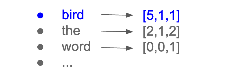
Consider the three following sentences from the well-known Surfin’ Bird song, and count the number of times each word appears in each sentence. Let’s first list all the words in the verses:

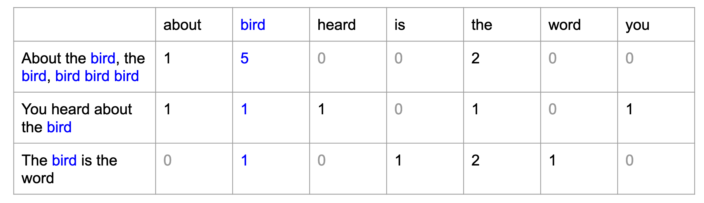
Each word is now associated with its own column of numbers, its own vector:

number of documents ∗ size of vocabulary

The vector size of each token equals the number of documents in the corpus. With this BOW approach, a large corpus has long vectors, and a small corpus has short vectors (as in the Surfin’ Bird example above, where each vector only has three numbers).

Create a Document-Term Matrix

The bag-of-words method is commonly used for text classification purposes, where the vector of each word is used as a feature for training a classifier. 

Consider the following sentences. The first two are about recipes, and the last three are about computing.

• Take 2 cups of flour.

• Mix the flour with the eggs.

• Replace your keyboard in 2 minutes.

• Do you prefer Windows or Mac?

• The MacBook Pro has such a noisy keyboard.

You can use the  CountVectorizer  from scikit-learn (read more on the official documentation page) to generate the document-term matrix with the following code:

# consider the following set of phrases
corpus = [
   '2 cups of flour',
   'replace the flour',
   'replace the keyboard in 2 minutes',
   'do you prefer Windows or Mac',
   'the Mac has the most noisy keyboard',
]

# import and instantiate the vectorizer
from sklearn.feature_extraction.text import CountVectorizer
vectorizer = CountVectorizer()

# apply the vectorizer to the corpus
X = vectorizer.fit_transform(corpus)

# display the document-term matrix as a dataframe to show the tokens


vocab = vectorizer.get_feature_names_out()
docterm = pd.DataFrame(X.todense(), columns=vocab)

It returns the document-term matrix:

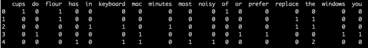
Each row corresponds to one of the sentences, and each column to a word in the corpus. For instance, the appears once in documents two and three and twice in document five, while the word flour appears once in documents one and two. The vocabulary is strongly related to the sentence topic: the word flour only appears in documents about recipes. On the other hand, the is less specific.

Reduce the Vocabulary of Your Corpus

The vocabulary is the set of all unique tokens in a corpus. Its size directly impacts the dimension of the document-term matrix. Therefore, reducing its size is essential to avoid performing calculations over gigantic matrices.

While removing stopwords and lemmatizing helps reduce the vocabulary size significantly, it’s often not enough.

Imagine that you are working on a corpus of 10,000 news articles with a total overall vocabulary of 10,000 tokens after lemmatization and removing stopwords. The corresponding document-term matrix would have a 10k by 10k dimension. That’s huge! Using such a matrix to train a classification model will lead to long training times and intense memory consumption.

Therefore, reducing the size of the vocabulary is crucial. The idea is to remove as many tokens as possible without throwing away relevant information. It’s a delicate balance that is entirely dependent on the context. One strategy can be to filter out words that are either too frequent or too rare. Another process involves applying dimension reduction techniques (PCA) to the document-term matrix. For a quick reminder about how PCA works, check out the OpenClassrooms course Perform an Exploratory Data Analysis.

Build a Classifier Model Using Bag-of-Words

Now that you know how to create a document-term matrix, let’s see how to apply it to text classification.

To recap, the typical machine learning process to train a classifier broadly follows these steps:

1. Feature extraction (vectorizing a corpus).

2. Split the dataset into a training (70%) and a testing (30%) set to simulate the model’s behavior on previously unseen data.

3. Train the model on the training set. In scikit-learn, this comes down to calling the   fit()  method on the model.

4. Evaluate the model’s performance on the test set, scored by a metric such as accuracy, recall, AUC (area under a curve), or by inspecting the confusion matrix.

In this chapter, we’ll focus on the feature extraction step, which, for NLP, equates to vectorizing a corpus. The goal is to demonstrate that it is possible to build a decent classifier model by counting the word occurrences in each document.

We will work on an excerpt of the classic Brown Corpus, the first million-word English electronic corpus created in 1961 at Brown University. This corpus contains text from 500 sources categorized by genre: news, editorial, romance, and humor, among others. We’ll only consider the humor and science fiction categories to simplify things.

The simplified dataset is available on the course GitHub repo and contains two columns: topic and text. Let’s load and explore it.

Load the Dataset

Load the dataset into a pandas DataFrame:

import pandas as pd
url = "https://raw.githubusercontent.com/alexisperrier/intro2nlp/master/data/brown_corpus_extract_humor_science_fiction.csv"
df = pd.read_csv(url)

print(df.topic.value_counts())

Returns:

humor              1053
science_fiction     948

The corpus holds 1053 humor sentences and 948 science fiction ones.

Here’s an example of sentences from each category taken at random from the corpus:

• science_fiction: “Through the telescope, Jack could see that both spacesuits were still attached to it .”

• humor: “They lay on the cellar floor in a disorderly pile.”

Now import spaCy and load a small English model:

import spacy
nlp = spacy.load("en_core_web_sm")

Preprocess the Data

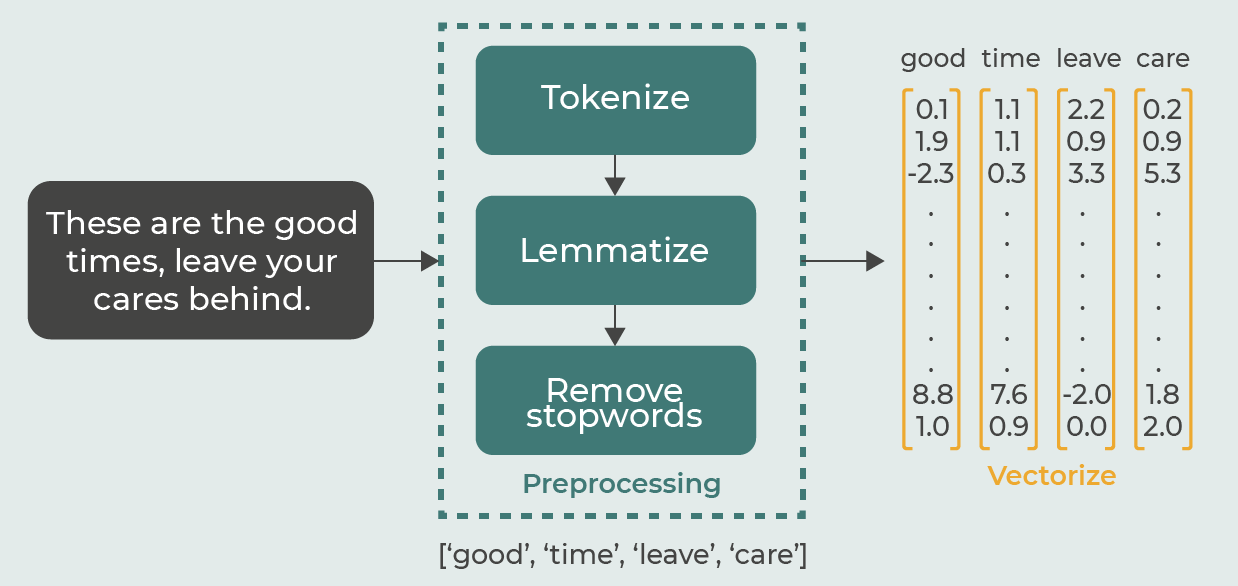
The preprocessing step consists of the different tasks you saw in Part 1:

• Tokenization.

• Removing stopwords.

• Lemmatization.

You can use spaCy to tokenize and lemmatize each text. Let’s define a simple function that processes each text with the spaCy model and returns a list of lemmatized tokens.

def lemmatize(text):
   doc = nlp(text)
   tokens = [token.lemma_ for token in doc]

   return tokens

Now, verify that the function works as expected.

text = "These are the good times, leave your cares behind."
lemmatize(text)

This returns:

['these', 'be', 'the', 'good', 'time', ',', 'leave', '-PRON-', 'care', 'behind', '.']

Seems correct, no?

But of course, the stopwords and punctuation signs haven’t been removed yet! spaCy makes stop word removal easy. It comes with a list of 326 predefined stopwords and a function   .is_stop  , which returns true when the token is a stopword. You can modify the   lemmatize()  function to filter out the tokens that are:

• Stopwords, using   .is_stop  .

• Punctuation signs, using  .is_punct  .

def lemmatize(text):

   doc = nlp(text)

   tokens = [token.lemma_ for token in doc if not (token.is_stop or token.is_punct)]

   return tokens

You can see that for the same sentence, “These are the good times, leave your cares behind,” you now get the following tokens:

['good', 'time', 'leave', 'care']

Much cleaner! 🧙

One last thing. Although it is possible to have a column type as a list in a pandas DataFrame, I have found that it is much easier to work with strings. You can use a scikit-learn vectorizer that works directly on the text and not on lists of tokens. Let’s modify the function one last time to return a string of all the tokens separated by spaces.

def lemmatize(text):

   doc = nlp(text)

   tokens = [token.lemma_ for token in doc if not (token.is_stop or token.is_punct)]

   return ' '.join(tokens)

That last version of   lemmatize()  applied to “These are the good times, leave your cares behind,” now returns:

'good time leave care'

Now apply the  lemmatize()  function to the whole corpus with:

df['processed_text'] = df.text.apply(lambda txt : lemmatize(txt))

The notebook contains extra steps to remove rows with few tokens. As you will see, you end up with 738 humor and 520 science fiction texts. You can find the notebook on the course GitHub repo.

Vectorize the Data

Now that the text has been tokenized, lemmatized, and stopwords and punctuation signs have been removed, the preprocessing phase is done. Next, we vectorize!

To vectorize the text, use scikit’s vectorizer methods. Scikit-learn has three types of vectorizers,  count  ,   tf-idf  ,  and  hash  vectorizers. The CountVectorizer counts the word occurrences in each document.

It takes but three lines of Python:

# import and instantiate the vectorizer
from sklearn.feature_extraction.text import CountVectorizer
cv = CountVectorizer()

# vectorize the lemmatized text
X = cv.fit_transform(df.processed_text)
print(X)

Returns:

<2000x4996 sparse matrix of type '<class 'numpy.int64'>'
 with 13243 stored elements in Compressed Sparse Row format>

X is now a sparse matrix of 1258 rows by 4749 columns. The number of columns corresponds to the size of the vocabulary. We could use the vectorizer parameters:   max_df  and  min_df  to filter words that are too frequent or rare.

Before training a model, the last step is to transform the topic columns into numbers. To do this, you arbitrarily choose 0 for humor and 1 for science fiction.

# transform the topic from string to integer
df.loc[df.topic == 'humor', 'topic' ] = 0
df.loc[df.topic == 'science_fiction', 'topic' ] = 1

# define the target variable as 0 and 1s
y = df.topic.astype(int)

For reasons beyond this course’s scope, Naive Bayes classifiers perform well on text classification tasks. In scikit-learn, you can use the MultinomialNB model:

from sklearn.naive_bayes import MultinomialNB
from sklearn.metrics import accuracy_score

# 1. Declare the model
clf = MultinomialNB()

# 2. Train the model
clf.fit(X, y)

# 3. Make predictions
yhat = clf.predict(X)

# 4. score
print("Accuracy: ",accuracy_score(y, yhat))

The performance of that model is really good with an accuracy score of:

Accuracy: 0.939

Lo and behold! 94% of the texts are correctly classified between humor and science fiction.

This is quite impressive. 🙂 But mostly because we trained the model on the whole corpus. In the companion notebook, we evaluate the model on unseen data and obtain 77% accuracy.

Let’s Recap!

• Vectorization is the general process of turning a collection of text documents, a corpus, into numerical feature vectors fed to machine learning algorithms for modeling.

• Bag-of-words(BOW) is a simple but powerful approach to vectorizing text. As its name suggests, it does not consider a word’s position in the text.

• Text classification is a classic use case of text vectorization using a bag-of-words approach.

• A document-term matrix is used as input to a machine learning classifier.

• Use spaCy to write simple, short functions that do all the necessary text-processing tasks.

The next chapter will look into another prevalent vectorization technique called tf-idf, which stands for term frequency- inverse document frequency. It is a variation of the bag-of-words approach, which is more efficient than simply counting word occurrences.