Transform Your Data Into Tables

Create a Table Using NumPy
Up to now, we’ve only seen one-dimensional tables and arrays, but it’s pretty rare to work with just a single column.
Let’s take an example. You work in the banking sector and you need to create a table that shows not just customer income, but also their monthly loan repayments, number of children and other information that could be useful.
Let’s consider the following customers:
Hugh is 21 years old, earns $1400 per month and has no children.
Richard is 54 years old, earns $2800 per month and has two children.
Emily is 27 years old, earns $3700 per month and has three children.
This data can be represented in the following table:
| Age | Income | Number of children |
Hugh | 21 | 1400 | 0 |
Richard | 54 | 2800 | 2 |
Emily | 27 | 3700 | 3 |
And here’s what the Python table would look like if we used a list:
hugh = [21, 1400, 0]
richard = [54, 2800, 2]
emily = [27, 3700, 3]
table = [hugh, richard, emily]
Let’s go through this together:
Firstly, for each of our bank's customers, we create a list containing all the information we have about that person.
Then we create a
tablelist to store the set of lists we previously created.
The table list contains three elements, which are themselves lists of three elements. So, what we have is a list of lists. However, we still have all the limitations relating to lists if we do it this way.
How else can we do it, though?
I bet you’re wondering! Well, once again, we’ll find a solution using NumPy and arrays.
An array is a multidimensional object, which means it’s possible to create arrays in all shapes and sizes, plus all the array methods take this multidimensional feature into account. Good, huh? Let’s try it out together!
The simplest way to create a table is to use a Python list of lists, as we would with a standard list. You just need to run the np.array(table) command to transform our list of lists into a NumPy array with three rows and three columns.
Let’s have a look at some more examples together to give you a better understanding of how it works:
tab1 = np.array([[1, 2],
    [3, 4],
    [5, 6]])

tab2 = np.array([[1, 2, 3],
        [4, 5, 6]])
These lines of code will generate:
a
tab1array, with three rows and two columns.a
tab2array with two rows and three columns.
As we did before, we can of course use NumPy functions to create tables of varying complexity. Here are a few examples of commonly used functions:
# A 3x5 table filled with 1s
np.ones((3, 5))
# a 4x4 table containing just 0s
np.zeros((4, 4))# a 6x3 table containing random values between 0 and 1
np.random.random((6, 3))# a 3x3 table filled with random integers from 1 to 10
np.random.randint(1, 10, size=(3, 3))Go ahead and try out some of these functions in your own environment. Change some of the values around to better understand how they work.
Discover the Similarity Between Arrays and Matrices
Do you remember when I mentioned that NumPy is a Python library designed specifically for carrying out complex scientific calculations? The tables we’ve seen up to now, taking the form of NumPy arrays, would be called matrices in the mathematical world. The initial aim of NumPy was actually to provide tools to handle matrices and perform matrix operations, before it began being used for a host of data applications.
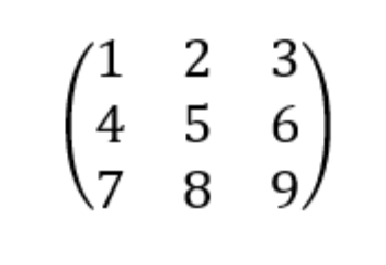
A matrix is a table of elements, as we’ve seen previously. We’d usually represent a matrix like this:
We regularly perform various operations on matrices. Let’s consider the following three matrices—A, B and C:
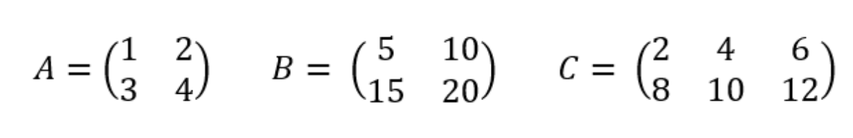
Since matrices A and B have the same dimensions (i.e., the same number of rows and columns), we can calculate the sum of (or difference between) matrices A and B by adding each corresponding element one by one:
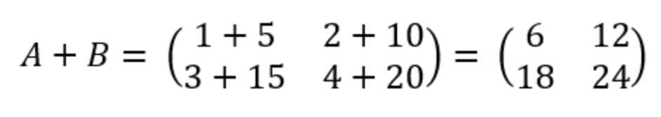
The same thing in NumPy:
A = np.array([[1, 2], [3, 4]])
B = np.array([[5, 10], [15, 20]])
C = np.array([[2, 4, 6], [8, 10, 12]])

A+B
It’s also possible to multiply elements one by one using the * operator, just as we would with a standard multiplication: A*B .
However, when we’re performing matrix calculations, we are much more likely to use what’s called the matrix product, or matrix multiplication. This is a fiddly calculation by hand—especially if we’re using matrices with large dimensions—but computers can handle it with ease.
With NumPy, matrix multiplication is performed using the @ operator: A@C . However, this operator is only available in Python 3.5 or above. Before this, we used the NumPy dot function to do matrix multiplication: AC = np.dot(A,C) . This function still works today, so you can choose which notation to use.
Understand Advanced Matrix Calculations
Do you remember when I told you that all array methods take into account the fact that arrays are multidimensional? Well, now let’s go into this in more depth in the following video. We’re going to see:
how to update an existing array.
how to access different array elements using the index.
some methods that could come in handy for scientific calculations.
There are of course many other methods available! The full list appears in the official NumPy documentation.
So, how about we put all this into practice?
Over to You!

Background
For this second task, we’ll continue working with our 10 bank customers, but this time we have three data items available for each:
Monthly income
Customer age
Number of children
Guidelines
Your objective is to use this information to create a NumPy table and respond to various requests from the loans department by manipulating the table using the techniques we’ve shown you throughout this chapter.
Please follow this link to the Transform Your Data Into Tables exercise.
Check Your Work
You can check your work against the exercise solution.
Let’s Recap
NumPy arrays are multidimensional. Based on the format of the data, they can be 2D, 3D or 4D.
You can create NumPy tables:
using the NumPy
arrayfunction to create a table from a Python list of lists:np.array(list_of_list).using predefined NumPy functions to populate a table with random values or a fixed value.
You can access elements from array A using the syntax
A[i,j], where i and j are the element’s row and column numbers within the table. The:operator lets you select several elements, including an entire row or column.There are many different methods that can be applied to arrays. The full list can be found in the NumPy official documentation.
In the mathematical world, these tables of numeric values are known as matrices. There are many algorithms that need to perform matrix calculations and if these are written in Python, they need to use NumPy.
Phew! Well, that was all a bit complicated, but we’ve managed to cover a few of the options available in NumPy. Once again, feel free to play around with the code to get to grips with it. It’s always easier if you practice!
Now let’s test your knowledge with a quiz.
