Perform an Exploratory Data Analysis

In the previous chapter, we used scikit-learn to carry out hierarchical clustering on the World University Rankings data. In this chapter, we will analyse the results.

Visualize the clusters

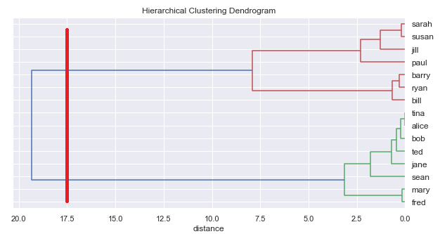
First, let's visualise the dendrogram of the hierarchical clustering we performed. We can use the  linkage()  method to generate a linkage matrix. This can be passed through to the  plot_denodrogram()  function in functions.py, which can be found in the Github repository for this course. 

Because we have over 600 universities, the dendrogram will be huge, so let's just visualise our smallest cluster. First, find the size of the clusters:

# Find the size of the clusters
X_scaled_clustered["cluster"].value_counts()

0 336
4 169
3 146
2 99
1 50
Name: cluster, dtype: int64

Now show the dendrogram for cluster 1, our smallest cluster:

# Show a dendrogram, just for the smallest cluster
from scipy.cluster.hierarchy import linkage, fcluster 
sample = X_scaled_clustered[X_scaled_clustered.cluster==1]
Z = linkage(sample, 'ward') 
names = sample.index 
plot_dendrogram(Z, names, figsize=(10,20))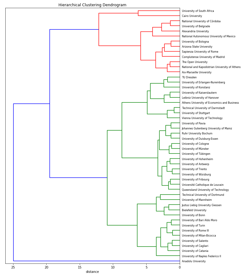

We can also visualise the clusters created by reducing the 10 dimensions to 2 dimensions and plotting the data points on the 2D space. We used this technique when we performed a k-means clustering.

First, perform the PCA, asking for 2 principal components:

from sklearn.decomposition import PCA

# Create a PCA model to reduce our data to 2 dimensions for visualisation
pca = PCA(n_components=2)
pca.fit(X_scaled)

# Transfor the scaled data to the new PCA space
X_reduced = pca.transform(X_scaled)

Now display the data points in their clusters:

display_factorial_planes(X_reduced, 2, pca, [(0,1)], illustrative_var = clusters, alpha = 0.8)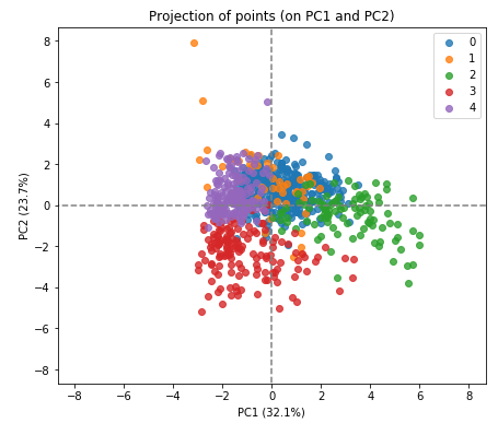

Interpreting the Meaning of the Clusters

But what do these clusters actually represent? As with k-means, the clustering algorithm has not given any indication as to what these 5 groups are. Again, we need to examine the clusters and determine a sensible way to interpret them.

Parallel Coordinates Plot

As we did with k-means, we can use a parallel coordinates plot to see how individual data points sit across all our variables. Here is the code to do that:

# Add the cluster number to the original scaled data
X_clustered = pd.DataFrame(X_scaled, index=X.index, columns=X.columns)
X_clustered["cluster"] = clusters

# Display parallel coordinates plots, one for each cluster
display_parallel_coordinates(X_clustered, 5)

However, as we saw with k-means, by characterising each group in a single data point we can sometimes get a clearer picture.  The k-means algorithm gave us the centroids, which we could use for this purpose.

The hierarchical clustering algorithm doesn't give us back the centroids, but we can compute them ourselves by taking the mean of each variable in each cluster:

means =  X_clustered.groupby(by="cluster").mean()

and then plotting:

display_parallel_coordinates_centroids(means.reset_index(), 5)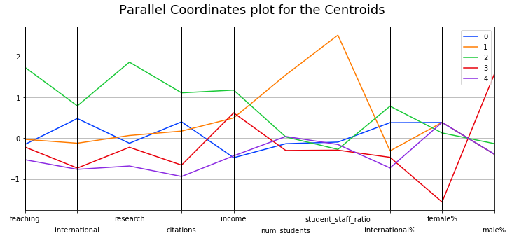

Box Plots

Another way to understand the clusters is to produce boxplots for each variable within each cluster:

X_clustered.boxplot(by="cluster", figsize=(15,10), layout=(2,5))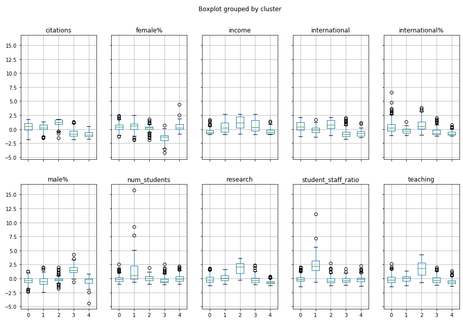

You might be able to see the same patterns emerging! For example, Cluster 2 is strong on teaching, research and international!

Which approach?

We have seen two different algorithms for clustering: k-means and hierarchical.  But which should we choose?  Here is some guidance.

Kmeans

The k-means algorithm converges in general very quickly. It is not uncommon for it to reach convergence after 10 iterations, even with many data points.

However, you can't guarantee to find the "optimal" set of clusters. The results depend on the initial set of centroids. This is why, generally, we run the algorithm several times and select the best result (the one with the smallest overall variance).

Also, k-means cannot determine the optimal number of clusters. It needs to be specified. However, again, we can run the algorithm several times, with different values of k, and identify at what point the intra-cluster distances don't improve significantly. This is the elbow method, which we saw earlier in the course.

Hierarchical

Hierarchical classification requires that distances between each and every point are calculated. If we have a large number of data points this can be very slow and require a lot of memory. Therefore, hierarchical clustering is best suited to small sample sizes.

However, unlike k-means, hierarchical classification does not require specifying a number of classes beforehand. We can ask the algorithm to generate the whole tree and then read off different numbers of classes.

Combined approach

It is possible to combine the best of both clustering approaches. For example, if you have a sample of 10,000 individuals, you can start by using k-means to group them into 50 clusters, extracting the 50 centroids, and then applying hierarchical clustering to these 50 centroids. With the dendrogram, you can choose the number of clusters (between 1 and 50) that suits you!

And That's a Wrap!

And there you have it: the tools you need to perform a successful multivariate analysis using PCA, k-means, and hierarchical clustering methods. Don't forget to test your skills in the final quiz, and remember to keep practicing the skills you have learned. Until next time! 

:magicien: