Perform an Exploratory Data Analysis

In the previous chapters, we looked at how a sample of individuals can be clustered using the k-means algorithm. In this chapter, we look at another clustering algorithm: hierarchical clustering.

How hierarchical clustering works

The algorithm is very simple:

Place each data point into a cluster of its own. 
LOOP
    Compute the distance between every cluster and every other cluster. 
    Merge the two clusters that are closest together into a single cluster.
UNTIL we have only one cluster

Example with one dimension

Let's look at an example using data with just one dimension, i.e. one variable. Here are the heights of 15 people:

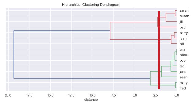
If we run the hierarchical clustering algorithm on the above data, we can plot the results on a diagram called a dendrogram:

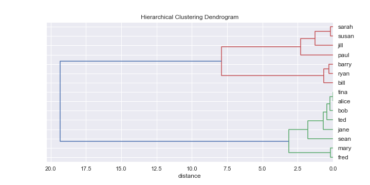
Let's take a look at what the algorithm did to produce the above diagram. The x-axis is the distance measure. Each name on the right is an individual placed in a cluster on its own. As we move to the left the lines show how the clusters have been joined together (or agglomerated).

The first line we encounter moving from right to left is the line joining Tina and Alice. Of all the individuals, they are closest in height:

In this case, the distance between the tina cluster and the alice cluster is 0.

Next, we have Mary and Fred:

In this case, the distance between the mary cluster and the fred cluster is 0.17.

Next, we find that the two closest clusters are the cluster of tina and alice and the cluster containing just bob:

In this case, the distance between the tina/alice cluster and the bob cluster is 0.2.

Next, we have this pair of clusters, with a distance of 0.22:

Next, we have these, with a distance of 0.29:

Then this group, with a distance of 0.49:

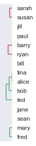
At this stage our clusters look like this:

We can continue using the above approach until we have just one cluster, represented by the final line on the left of our dendrogram.

Moving up to 2 or more dimensions

The above example has just one variable, or one dimension. As you know by now (:honte:), when we talk about measuring the distance between data points, we can apply the same maths to two or more dimensions.

Reading off the number of clusters

One of the advantages of hierarchical clustering over k-means clustering is that when we generate the cluster hierarchy, we have generated a full tree all the way from every data point in its own cluster up to a single cluster.

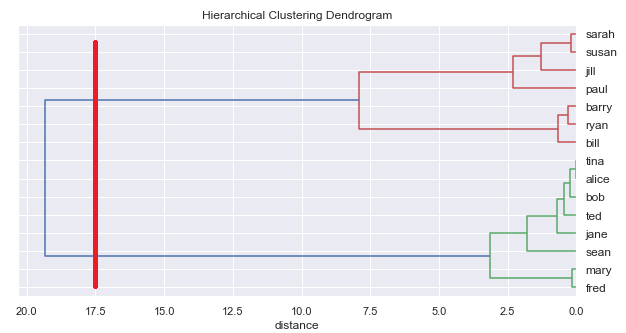
For example, with our example above, we could read off 2 clusters:

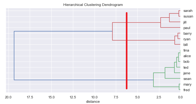
Or we could read off 3 clusters:

or 5:

Terminology

There are two important choices we made about how this algorithm proceeded:

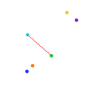
• 1. We decided that our measure of distance between two data points would be the Euclidean distance.  So, for example, we can measure the Euclidean distance between the blue and green points in the plot below:

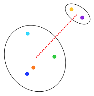
• 2. We decided that when we have a cluster of data points (e.g. tina/alice/bob) that the distance between the cluster and another cluster (e.g. ted) is the total variance of the resultant cluster. In other words, we place all the data points from the two clusters into a single cluster and calculate the variance of this single cluster.  This is called the Ward linkage criterion.  So, for example, we can measure the distance between the two clusters shown below by computing the variance for all 6 points in the clusters:

Other choices can be made for computing these distances, but for our investigation, we will stick with these.

Recap

• Hierarchical clustering generates a full tree all the way from every data point in its own cluster up to a single cluster

• We can run the algorithm once and then read off as many clusters as we want - no need to determine the number of clusters from the beginning