Assess Linearity
Now that you have a better understanding of what linear regression is, and how it applies to companies across industries and departments, let's dive into the first important concept behind it: linearity.
Linearity is, of course, at the heart of linear regression and its variants. It is a simple and elegant property widely used in forecasting, neural networks, and many other complex machine learning algorithms. As you will see, it is a very robust element of data analysis.
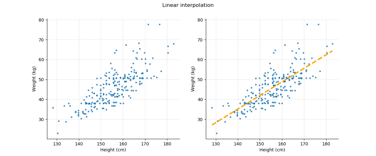
You probably already have a good idea of what linearity is. When asking to define it, the answer usually involves the idea of a straight line that best fits the samples. For instance, plotting the weight versus the height of a sample of school children gives us the figure below on the left. The goal of linear interpolation is to find the straight line that is closest to all the points in the graph.
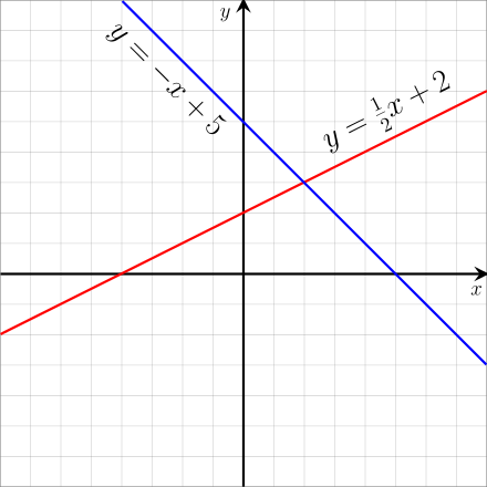
And to refresh your memory, the general equation of a line is:
is the classic equation for a line in the two-dimensional (2D) plane. is the slope, is the constant, and for different values of and we obtain different lines as illustrated by the figure below.
The True Definition of Linearity - and a Catch
Let's go back to the mathematical definition of linearity of a function. Consider a function where is a real number (also called a scalar). The exact mathematical definition of a linear function is the following:
is a linear function if, and only if, it verifies these two conditions:
The first condition is called the multiplicative property:
for whatever number
The second condition is called the additive property:
That's it! It is quite a simple but powerful definition.
You can also verify that a line corresponds to a linear function. Let's start with the equation of a line that goes through the origin point (0,0):
When the slope , the line goes up, and when , the line goes down. And since , all the lines generated by go through the origin point with coordinates .
You can verify the multiplicative property:
And the additive property:
The Catch
What about lines that do not go through the point of origin? Lines whose equation is:
with
In that case, you can verify that the function is not linear, at least not according to the strictest definition of linearity. You have:
You can also verify that as an exercise. :lol:
The presence of the constant breaks the two conditions required to make the function linear.
Linear functions that respect the additive and multiplicative properties are called homogeneous linear functions.
And now for some nonlinear functions!
Nonlinear Functions
What is a nonlinear function?
Any function that does not rely only on multiplication and addition is nonlinear.
Examples of nonlinear functions include:
This function does not verify the additive or the multiplicative property. Let's verify the additive property:
is nonlinear since
similarly is also nonlinear for the same reason:
You get the drift.
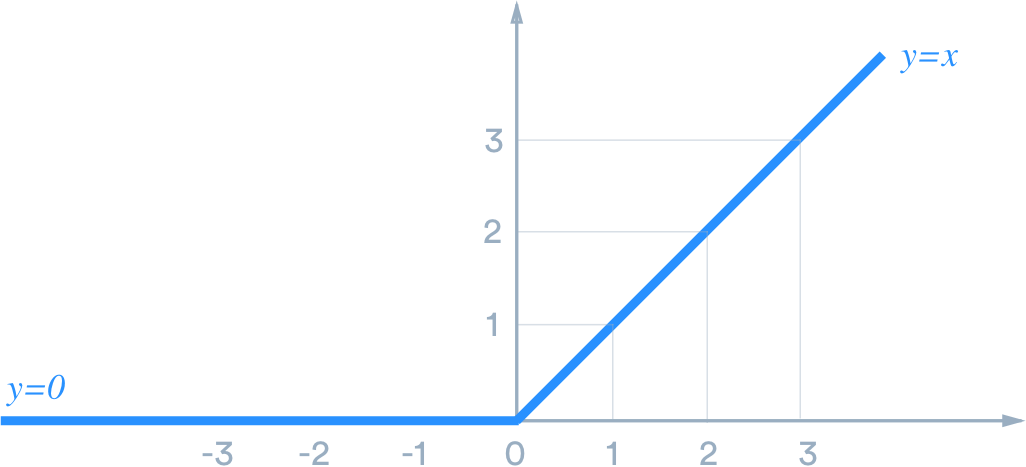
The next function is also nonlinear, although it is linear on each segment defined by being negative or positive.
The function spanning negative and positive values of x is nonlinear. This function is called a rectified linear unit (ReLU) is it an activation function widely used in deep learning to introduce nonlinearities in the neural network.
Multi-Dimensions
So far, we have only worked with real numbers. The linearity property of a function can extend to vectors.
A vector of dimension N is simply a set of N numbers taken together as a single object.
In the 2D plane, a vector has 2 numbers . In a 3D volume, a vector has 3 numbers and so forth. Generalizing to N dimensions, a vector has N numbers
To multiply two vectors with , simply write:
The function defined as where and are both dimensional vectors is a linear function in the strictest sense of the definition.
Application to Linear Regression
Consider the relations between , our target variable, and two predictors, and .
In this example, is the weight of a middle school student, is the age, and the height. You can imagine that there's a linear relationship between the weight of the student and his/her age and height and write:
Where are coefficients we would like to estimate.
You can rewrite the above equation as a vector equation:
With the vector
Here, you have a linear function with two variables.
If there were more than two predictors of the student's weight but, instead predictors, the equation of the weight as a linear function of all the N predictors would still take the form where would now be a vector of coefficients and a vector of predictors.
Why is Linearity so Important?
What's interesting about linear function is that the linear feature is conserved by linear transformations:
The sum of two linear functions is still a linear function.
The multiplication of a linear function is also a linear function.
The composition of two linear functions is a linear function.
The last point means that if two linear functions are defined by and , the composition of g and f : is still linear! Linearity is very meta. :)
This means that if you apply linear regression to a dataset, you can transform your variables and still be in the same context of linear functions. Even when your dataset shows some strong nonlinearities.
Linear Modeling of Nonlinearities
The linear model can also extend to model nonlinearities in the data.
Let's say you want to include the height as a predictor of the school children's weight as well as the square of the height. Although the square of the height is not a linear function of the height, you can still build a linear model as such:
This is a linear model with respect to two variables: and . We have simply created a new predictor and used it in the linear model.
Is My Data Linear?
How do you know if the relation between your variables is linear? The question is whether there is a linear relationship between one or several of your predictors and the target variable.
One way to check the linearity is to plot the target versus the predictors for each of the predictors in the dataset.
If the plot shows a distinct trend, you can conclude that there is some amount of linearity between the two variables. When the plot shows a different pattern, the relation is not linear.
The following plot shows the relation between the weight and the height in school children. The straight line is the linear interpolation of the data.
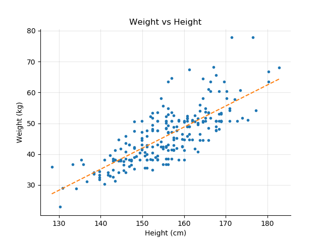
As expected, the weight increases with the height. Although not perfect, the relationship between the two variables shows some degree of linearity.
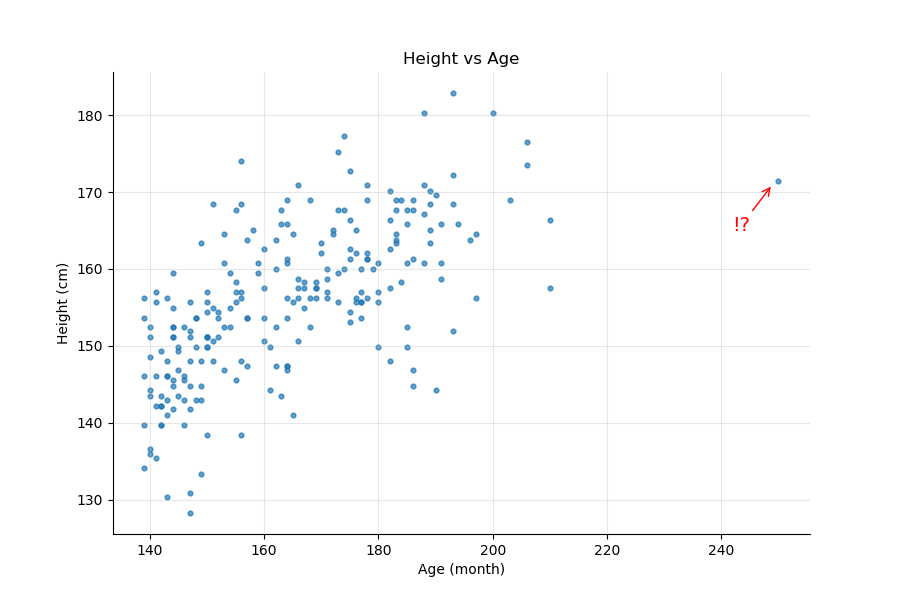
If you look at the height versus the age, the linearity of the relationship is less obvious as shown by the following figure:
The auto-mpg dataset is another dataset we're going to work with throughout the course. The original dataset comes from UCI Machine Learning repository. The auto-mpg dataset lists the fuel consumption in miles per gallon for over 300 cars from the 80s. Each sample has information on acceleration, displacement, weight, and some categorical variables. We'll come back to that dataset later in the course.
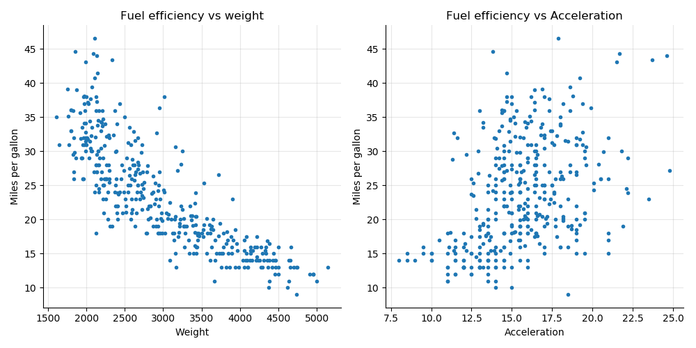
For now, let's look at the variables weight and acceleration with respect to the fuel efficiency/ miles per gallon (mpg) target variable.
The plot below on the left shows the mpg versus weight and on the right the mpg versus acceleration. As expected, the heavier the car, the worse its fuel consumption (lower number of miles per gallon).
The plot on the left shows a distinct decreasing relation between mpg and weight. Some degree of linearity exists between the two variables.
The plot on the right is hardly interpretable as a linear relation. The points form a sort of central blob, and it would be unwise to infer anything from it.
Looking at plots to assess the linearity of the relation between two variables is fine, but it does not give you enough information on the degree of that linearity. How close is the relation to a single straight line?
At this point several important questions are left unanswered:
How can you effectively measure the degree of linearity?
How can you be certain that a linear model properly captures the information contained in the dataset?
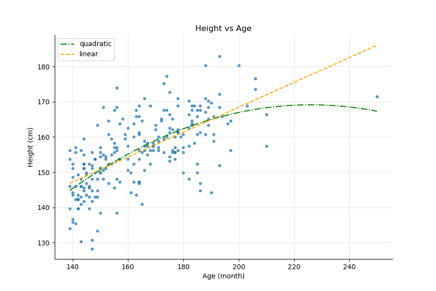
To illustrate that last point, let's look at the Height vs. Age plot above. If you trace a linear interpolation and a quadratic one (the curved line) on the same graph, how do you know which interpolation is better? Furthermore, the point on the right seems to have a big impact on the quadratic line, but by how much? What would happen if we removed it?
Summary
Linearity is central to this course as well as a wide range of techniques with many diverse application domains, from forecasting and time series to neural networks, signal processing, and modeling of natural phenomena.
In this chapter, we covered the following key elements:
A strict and mathematical definition of linearity based on additive and multiplicative properties.
That linear functions deal with scalars as well as vectors with the same simple expression
That assessing the linearity between two variables can be done visually, but the conclusion is not always obvious or unique.
Looking back at the plots in this chapter, two types of relations between variables emerge:
One where the plot shows a swarm of points, with no distinguishable patterns; a blob of point. This was the case for the Mpg vs. Acceleration plot.
Other plots where some patterns can be distinctively observed, such as the Weight vs. Height in schoolchildren plot.
