Design Effective Statistical Models to Understand Your Data

Hypothesis testing is a statistical method that helps decide if the observation of a variable can be trusted. Observation of a variable means making a measurement or assuming some property of the variable based on a finite number of samples. 

The observation can be:

• A measure: mean, median, standard deviation, percentile, etc.

• A comparison between two populations: correlation, difference in means, etc.

• Some intrinsic characteristic of the variable: is normally distributed, stationary, etc.

Hypothesis testing is commonly used across many industries and drives a wide range of statistical tests. It's also at the center of model selection and interpretation in linear and logistic regression!

In this chapter, we start with an overview of hypothesis testing. We then apply different statistical tests to our school and auto-mpg datasets to illustrate hypothesis testing and understand its strength and shortcomings

Overview

Let's start with an example!

The school dataset has the height, weight, and age of 237 school children but also their gender with 111 girls and 126 boys. It would be interesting to compare the height of boys and girls and see if the difference is statistically significant.

If you take the height average from the sample dataset, you have:

$\$\backslash [\{\backslash hat\; H\_\{boys\}\}\; =\; 157.74\; \backslash \backslash \; \{\backslash hat\; H\_\{girls\}\}\; =\; 153.74\backslash ]\$$

Boys seem taller on average than girls, though not by much. The difference is only 4 cm. Is that difference statistically significant?

This is where hypothesis testing can help. The general idea is to calculate the probability that your observation is due to some random factor. When that probability is small, you conclude that the observation can be trusted.

Imagine that you want to assess that girls and boys don't have the same average height                     ( $\$\backslash (\backslash hat\; H\_\{boys\}\; \backslash neq\; \backslash hat\; H\_\{girls\}\backslash )\$$ ) using the schoolchildren example. Therefore, you want to be able to reject the null hypothesis that girls and boys have the same average height.

You have the null hypothesis:  $\$\backslash (H0:\; \backslash hat\; H\_\{girls\}\; =\; \backslash hat\; H\_\{boys\}\backslash )\$$ 

You would like to reject in favor of the alternative hypothesis:  $\$\backslash (H1:\; \backslash hat\; H\_\{girls\}\; \backslash neq\; \backslash hat\; H\_\{boys\}\backslash )\$$ 

To compare the means of two different populations, use the t-test. The Python SciPy library has a t-test function. The documentation indicates that:

scipy.stats.ttest_ind(a, b, ...)

Calculate the t-test for the means of two independent samples of scores.
This is a two-sided test for the null hypothesis that two independent samples have identical average values.

Let's open the dataset and collect the heights of girls and boys in an array:

import pandas as pd
df = pd.read_csv('school.csv')
G = df[df.sex == 'f'].height.values
B = df[df.sex == 'm'].height.values

Applying the t-test to the two populations boils down to these two lines of code:

from scipy import stats
result = stats.ttest_ind(G,B)
print(result)

The result is:

Ttest_indResult(statistic=-3.1272160497574646, pvalue=0.0019873593355122674)

Since the p-value is smaller than the standard threshold of p=0.05, you can reject the null hypothesis of equal averages. The conclusion is that, regarding the schoolchildren population, boys are not the same height as girls.

Did You Notice?

You probably noticed that we did not conclude that boys are taller than girls because we did not define the null and alternative hypothesis as:

$\$\backslash (H0:\; \backslash hat\; H\_\{girls\}\; \backslash gt\; H\_\{boys\}\; \backslash \backslash \; H1:\; \backslash hat\; H\_\{girls\}\; \backslash le\; H\_\{boys\}\backslash )\$$

Another Example

Here's the code:

average_weight_girls = df[df.sex == 'f'].weight.mean()

You may have noticed that the t-test returns values with two values: statistic and p-value. Let's take a look at both of these below.

The P-Value

The p-value is the probability of the observation, assuming that the null hypothesis is true.

This is graphically illustrated by:

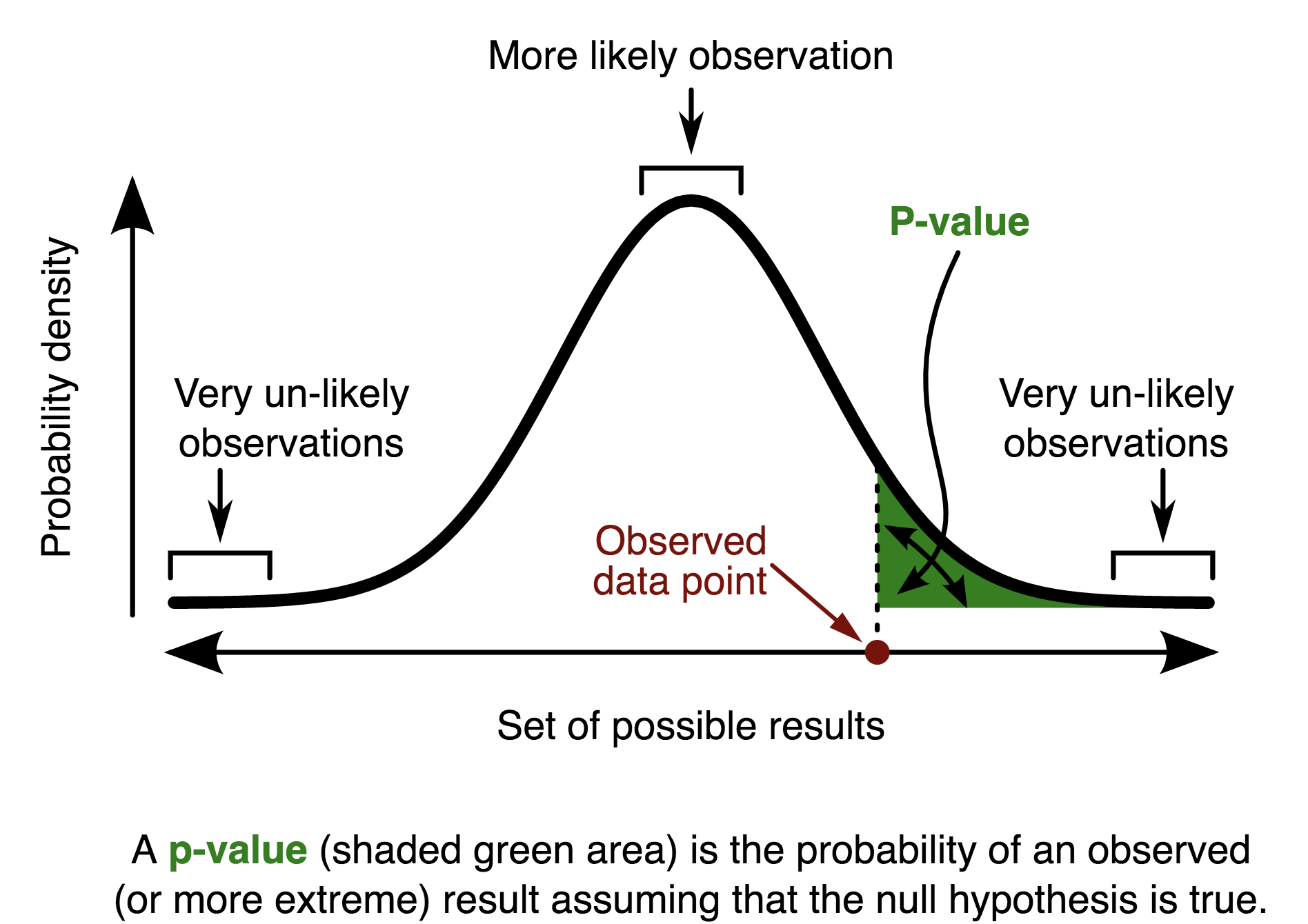
Graphic by Chen-Pan Liao from wikimedia.org

This graph shows the probability distribution of observation for a given statistical test, assuming the null hypothesis in the special case, where that probability distribution is normal. When the probability distribution is known, it possible to calculate its percentiles and confidence intervals. The standard 0.05 p-value threshold corresponds to the 95% confidence interval of the probability distribution.

The T-Test Statistic

The t-test returns another value: the statistic. What is that?

In statistics, a statistic is just another name for a measure or calculation. The average, the correlation, and the median are all statistics.

So What Did We Do Here?

In practice, the way hypothesis testing works is a bit of a mind twister:

1. Start by choosing the adequate statistical test (we chose the t-test).

2. Then define the hypothesis you want to reject, calling it the null hypothesis.

3. Calculate the p-value, which is the probability of the observation assuming this null hypothesis.

4. When the p-value is small, reject the null hypothesis.

The hypothesis that what you observe happened by chance is the null hypothesis and is noted $\$\backslash (H\_0\backslash )\$$ .

The opposite hypothesis is called the alternative hypothesis and is noted $\$\backslash (H\_1\backslash )\$$ .

The probability of the observation, assuming the null hypothesis is true, is called the p-value.

If the p-value is below a certain threshold, usually p=0.05, you can conclude that the null hypothesis is unlikely to be true and reject it; thus, adopting the alternative hypothesis when both are mutually exclusive.

Good question! Let's look at that next.

Testing for Normality

Here's another example of hypothesis testing; this time, assessing the nature of the distribution of a variable.

Plotting the histogram and probability distribution of the variable acceleration from the auto-mpg dataset is demonstrated on the following graph:

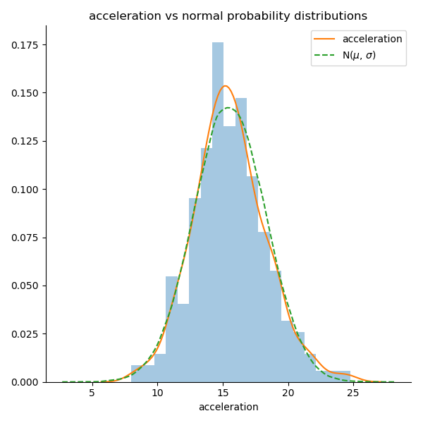
Compared to the distribution of a normal distribution, the two plots look very similar. So it looks like the acceleration variable is normally distributed, but is it? How confident of that conclusion are you just looking at the graph? This is a question that hypothesis testing can help answer.

Normal Distribution

But first, a quick word on the normal distribution.
A variable is said to follow a normal distribution when it is shaped like a bell curve:

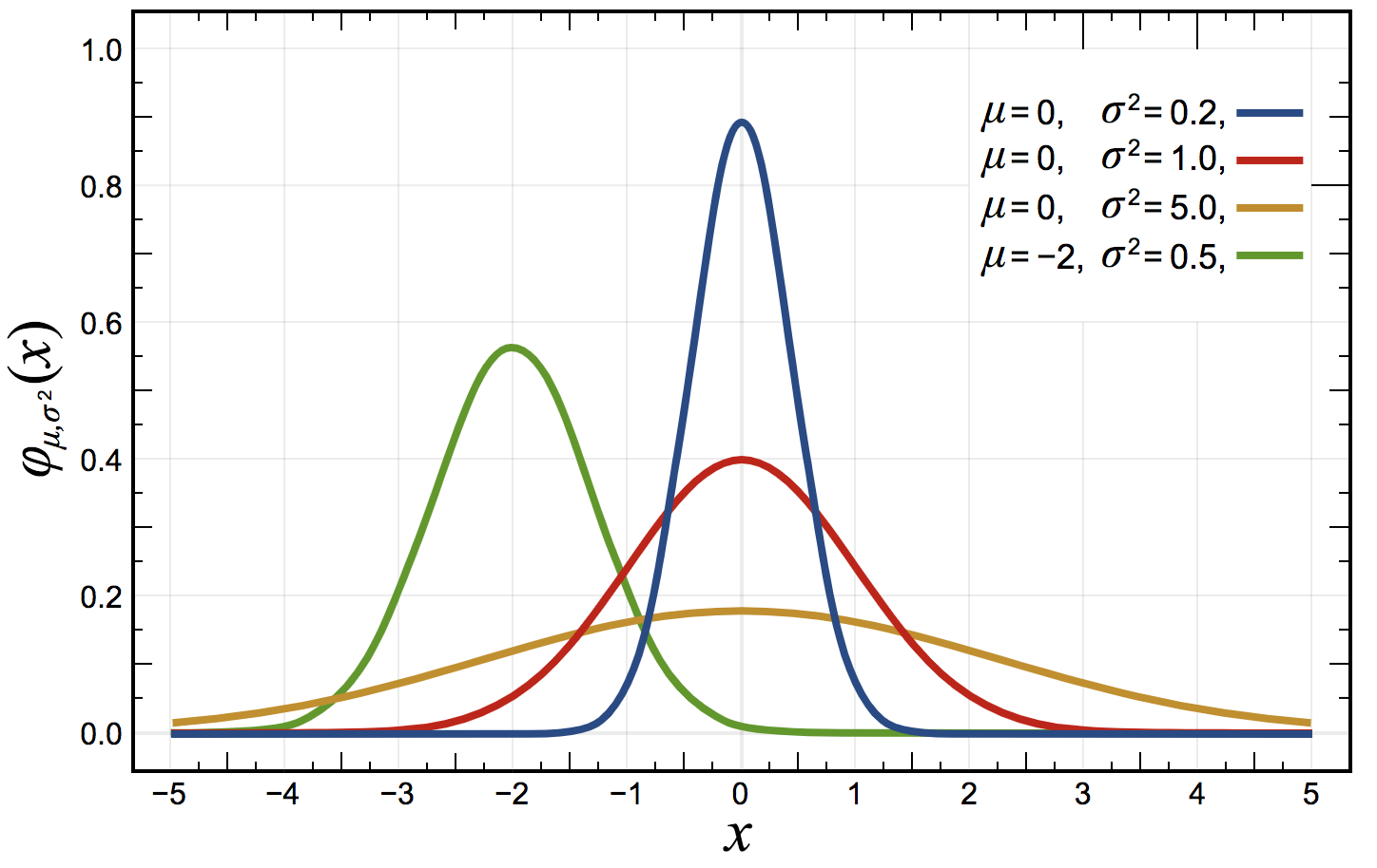
A more formal mathematical definition is that the probability density of the normal distribution is:

$\$\backslash [f(x\backslash mid\; \backslash mu\; ,\backslash sigma\; ^\{2\})=\{\backslash frac\; \{1\}\{\backslash sqrt\; \{2\backslash pi\; \backslash sigma\; ^\{2\}\}\}\}e^\{-\{\backslash frac\; \{(x-\backslash mu\; )^\{2\}\}\{2\backslash sigma\; ^\{2\}\}\}\}\backslash ]\$$

Where $\$\backslash (\backslash mu\backslash )\$$ is the mean or expectation of the distribution (and also its median and mode), and $\$\backslash (\backslash sigma^2\backslash )\$$ is the standard deviation. A variable that follows a normal distribution of mean  $\$\backslash (\backslash mu\backslash )\$$ and variance  $\$\backslash (\backslash sigma^2\backslash )\$$ is noted:

$\$\backslash [X\; \backslash sim\; \backslash mathcal\{N\}(0,\; 1)\backslash ]\$$

The normal distribution is omnipresent in statistical and machine learning. It possesses many elegant and efficient properties.

Normality Test

A common way to test the normality of a variable is the Kolmogorov-Smirnov test for goodness of fit. The Kolmogorov-Smirnov tests the null hypothesis that two distributions are identical.

Here we will test the hypothesis that the acceleration variable and a normal distribution of similar mean and variance are identical.

So, in this case, the null hypothesis is the observation that we want to verify. If the data shows that we should reject the null hypothesis, we conclude that our data is not normally distributed.

In the following Python script, open the auto-mpg dataset and apply the Kolmogorov-Smirnov test (KS) from the SciPy library (documentation). The KS test takes the empirical data and the name of a standard distribution in our case. The test assumes that the sample distribution is centered and of variance 1, so you need to center and normalize the data to be able to compare it to an N(0,1) distribution.

You do so with the following operation:  

from scipy import stats

The result is:

Since the p-value is well above the 0.05 threshold, you cannot reject the null hypothesis.

The conclusion is that the p-value, i.e., the probability of observing our data under the assumption that the data follows a normal distribution, is high enough to be trusted.

Your Turn!

Check out the solution in the following screencast:

Words of Caution

Once you get around the logic behind hypothesis testing, the method seems simple enough. Depending on the p-value, you reject the null hypothesis or not. But there are several shortcomings of that method mostly due to a misinterpretation of the results.

Population Bias

In the first part of this chapter, we concluded that on average, boys are taller than girls based on a dataset of 237 samples of schoolchildren. This conclusion only applies to our dataset, and cannot be directly generalized to a more global population without more statistical evidence and analysis.

For instance, if the boys in this school were all basketball players, and taller than the normal population, then our dataset would be biased. Hidden biases in the dataset are always something to look for and test for when possible.

Truth and Rejecting the Null Hypothesis

One common abuse of hypothesis testing is that rejecting the null hypothesis directly implies that the observation is true.

Rejecting the null hypothesis means that every other possibility may be true. For instance, if you test that a variable follows a normal distribution centered of variance 1.

The null hypothesis is:  H0:X∼(0,1)

If $\$\backslash (H\_0\backslash )\$$ is rejected, that means that several things could be true:

• The mean is not 0.

• The variance is not 1.

• The distribution is not normal.

What Is the Correct Interpretation of the P-Value?

The p-value is often interpreted as the probability of the null hypothesis ( $\$\backslash (p(H\_0)\backslash )\$$ ), which is not entirely true. The p-value is the probability of the observation assuming the null hypothesis                ( $\$\backslash (\backslash text\{p-value\}\; =\; p(X\; /\; H\_0)\backslash )\$$ ). In probability theory land, you write that the p-value $\$\backslash (p(X\; /\; H\_0):\backslash )\$$

$\$\backslash [p(X\; /\; H\_0)\; \backslash neq\; p(X)\; \backslash \backslash \; p(X\; /\; H\_0)\; \backslash neq\; p(H\_0)\; \backslash \backslash \; p(X\; /\; H\_0)\; \backslash neq\; p(H\_0\; /\; X)\backslash ]\$$

P-Hacking

But there's more, and it's called p-hacking!

By running repeated experiments on the same datasets but different chunks of the dataset, there's bound to be a subset of samples for which the p-value is lower than 0.05. This is called p-hacking: running an experiment many times until the p-value is low enough so you can reject the null hypothesis and claim that the observation is real. 

P-hacking is superbly illustrated in this comic from XKCD. A scientist tests the impact of jelly beans on acne and defines the null hypothesis as, "There's no link between jelly beans and acne." He then tests all the possible colors, each time with a p-value > 0.05, until one day, testing green jelly beans, the p-value is below 0.05. The scientist happily concludes that "green jelly beans cause acne."

There's a push back by many scientists on hypothesis testing and the concept of statistical significance. The claim is that it is too easy to hack and often leads to erroneous conclusions.

However, hypothesis testing is widely used for all types of problems and data analysis and is far from being discarded as a reliable method for statistical analysis.

Summary

In this chapter, you learned about hypothesis testing, a key method in statistics.

The key takeaways from this chapter are:

• Hypothesis testing involves four steps:

  • Select the right statistical test and rejection threshold.

  • Define a null hypothesis and an alternative one.

  • Apply the test on the data.

  • Decide to reject the null hypothesis or not based on the p-value.

• Use the t-test to compare means of two samples of the same data.

• Apply the Kolmogorov-Smirnov test to assess that a variable is normally distributed.

• A statistic is a calculation based on the data.

• The p-value is the probability of our observation, assuming the null hypothesis and is not the probability of the null hypothesis.

This concludes the first part of the course. You are now ready to build linear regression models.