Design Effective Statistical Models to Understand Your Data

You now understand the three main concepts which are required to build linear regression models: correlation, linearity, and hypothesis testing.

In this chapter, we will apply these concepts to build linear models between variables!

The advertising dataset contains 200 samples with amounts spent on three different media channels: newspaper, radio, and TV. The sales variable is the outcome. Our goal is to understand how spending amounts on each one of these channels influence sales. We start with univariate regression, building linear models between the target variable sales and one input variable at a time. This will allow us to analyze the results in detail, and learn which media is the most efficient to increase sales.

By the end of this chapter, you will be able to:

• Build a regression model (between sales and its most correlated media variable).

• Interpret the results of the regression using R-squared, p-values of the coefficients, and the t-statistic.

Let's get to work!

The Dataset

This advertising dataset is a classic one in statistical learning. It is analyzed in an excellent book called Introduction to Statistical Learning by James, Witten, Hastie, and Tibshirani, available online for free.

The dataset consists of 200 samples with four variables:

• Advertising budgets for newspaper, TV, and radio (the predictors)

• Sales (the outcome)

      TV  Radio  Newspaper  Sales
0  230.1   37.8       69.2   22.1
1   44.5   39.3       45.1   10.4
2   17.2   45.9       69.3    9.3
3  151.5   41.3       58.5   18.5
4  180.8   10.8       58.4   12.9

Visualization

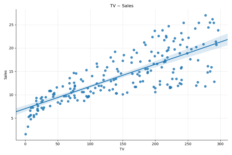
Start by plotting each input variable to the outcome variable.

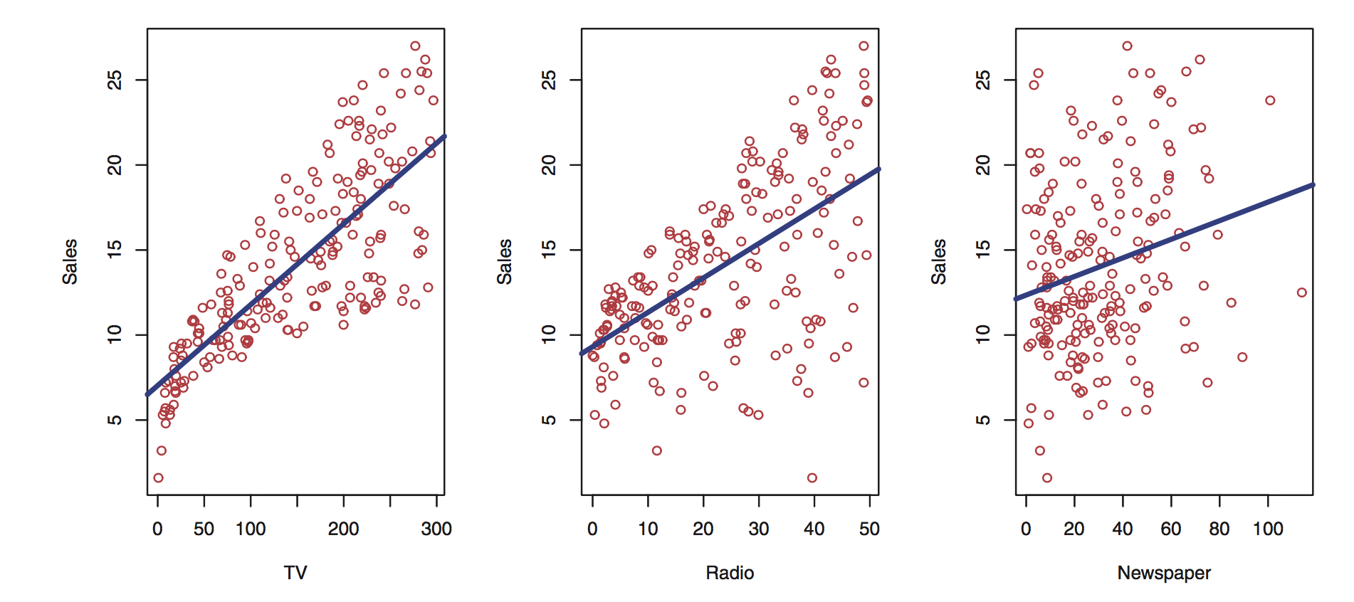
You can already infer some information from these plots:

• As TV and radio spending increase, so do sales.

• Newspaper spending impact on sales is less pronounced, although there is a trend.

• It looks like TV spending is more efficient than radio as the overall trend of the plot is steeper.

Calculating the correlation between the variables gives:

df = pd.read_csv('advertising.csv')
df.corr()['Sales']

TV 0.782224
Radio 0.576223
Newspaper 0.228299
Sales 1.000000

Which confirms what we inferred from the plots above.

Univariate Linear regression

As mentioned above, univariate linear regression is when you want to predict the values of one variable from the values of another. Let's start by building a linear model between sales and TV, which is the variable most correlated with the outcome.
We want to find the best coefficients a and b such that:

$\$\backslash [Sales\; =\; a\; *\; TV\; +\; b\backslash ]\$$

For that, we turn to the statsmodel library in Python, which can be installed with:

pip install statsmodels

or

conda install statsmodels

Sales ~ TV

To build a linear model between sales and TV, use the method called ordinary least square, or OLS. In short, the OLS method will find the line closest to all the points of the plot as shown:

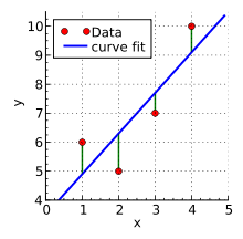
We will come back to the inner workings of the OLS method later on.

The following is the code to build and fit the linear regression model to the data:

# import the modules
import statsmodels.api as sm
import pandas as pd

# Load the dataset
df = pd.read_csv('advertising.csv')

# single out the input variables X 
X = df['TV']
# Add a constant 
X = sm.add_constant(X)
# define the target variable y
y = df['Sales']

# Define the model
model = sm.OLS(y, X)

# Fit the model to the data
results = model.fit()
print(results.summary())

Which gives the following output:

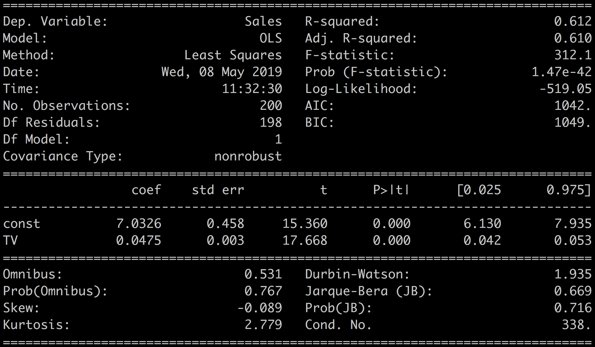
Let's break this down. For a start, we will only focus on a few of the metrics in this chapter. The rest we will save for later.

The most important element of the results is the line with the values for the coefficients, p-value, and confidence intervals:

The metric R-squared: 

Code Review

But first, let's go over the code above and explain what we did. Two things need our attention: formatting the input variables into X, and fitting the model.

We first select the predictor variable, in our case TV:

X = df['TV']

X is an array of 200 samples  x = [x_1, x_2, ... , x_N]^T. If you feed that vector to the OLS method, it will try to find the best line that corresponds to:

$\$\backslash [Sales\; =\; a\; *\; X\backslash ]\$$

This line goes through the origin point and does not have a constant term. However, you want to find the best line, the best parameters a and b, that fits:

$\$\backslash [Sales\; =\; a\; *\; TV\; +\; b\backslash ]\$$

For that, you need to add a constant vector to df['TV'] so that X becomes an array of dimension 2,N:

X = [[1,x_1],
     [1,x_2],
     ...
     [1,x_N]]

Use the  add_constant  method in statsmodel:

X = sm.add_constant(X)

If you visualize the shape and head of X before and after, you get:

X = df['TV']
print("before: X shape: {}".format(X.shape))
> before: X shape: (200,)

X = sm.add_constant(X)
print("after: X shape: {}".format(X.shape))
> after: X shape: (200,2)

A const column has been added to X. Next, define a simple OLS model based on that data:

model = sm.OLS(y, X)

And call the  fit()  method to fit the model to the data:

results = model.fit()

Finally, print the summary of the results with  print(results.summary()).

Interpreting the Results

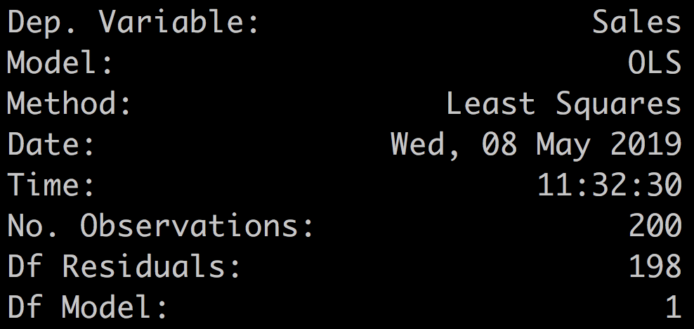
The upper-left quadrant of the results are mostly a summary of the method indicating the name of the outcome variable (here,  Dep. Variable ), which is  sales; the  model,  OLS; the  method,  least squares; and the  number of samples (here,  No. Observations),  200.

Before we look more closely at the numerical results, we can plot the line estimated by the OLS method with the  results.fittedvalues  method. As its name indicates, the fitted values can be obtained from the regression coefficients:

results.fittedvalues = results.params['TV'] * df['TV'] + results.params['const']

You can also access the residuals, i.e., the error between the real values and the fitted values.

results.resid = df['Sales'] - results.fittedvalues

For ease of manipulation, let's add the fitted values to the initial DataFrame.

df['fitted'] = results.fittedvalues

To plot the fitted values versus the real values,  sort the DataFrame. This is just for plotting convenience.

df.sort_values(by = 'TV', ascending = True, inplace = True)

Then plot the fitted values and the residuals with:

plt.scatter(df.TV, df.Sales, label = 'Sales' )
plt.plot(df.TV, df.fitted, label = 'Fitted' )
plt.legend()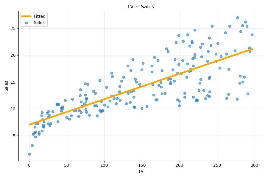

Coefficients

Let's focus on the coefficients and related statistics:

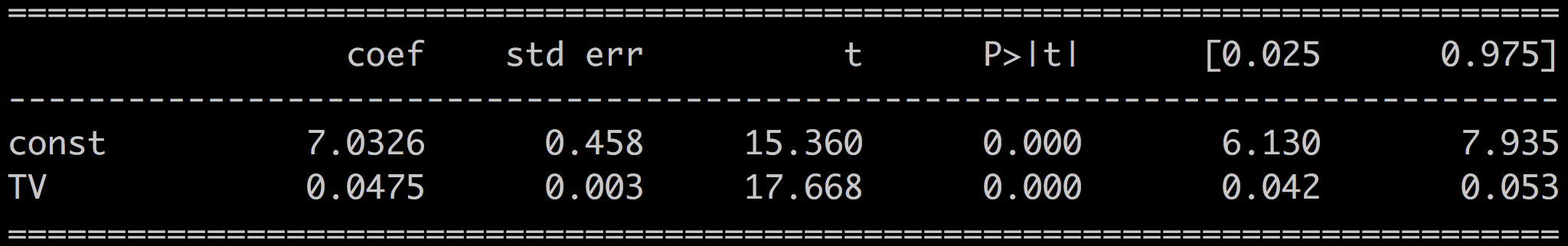
The  coef  is the coefficient value in the equation:

$\$\backslash [Sales\; =\; coef\_\{TV\}\; *\; TV\; +\; coef\_\{Const\}\backslash ]\$$

In our case, we have:

$\$\backslash [df.Sales\; =\; 0.0475\; *\; df.TV\; +\; 7.0326\backslash ]\$$

P-values

Next, the  P>|t|  value is the p-value associated with the coefficient. The p-value for each coefficient tests the null hypothesis that the coefficient is equal to zero (no effect). The full values of the p-values can be obtained with:

print(results.pvalues)
const 1.406300e-35
TV 1.467390e-42

You can see here that the p-values are well below the standard threshold of 0.05. You can, therefore, reject the null hypothesis and conclude that the coefficient values are relevant given the data.

T-Statistic and Standard Error

• The standard error is an estimate of the variations of the coefficient.

• The t-statistic is the coefficient divided by its standard error.
   $\$\backslash (t\; =\; \backslash frac\{coeff\}\{Std\; Err\}\backslash )\$$

The t-statistic is a measure of the precision with which the regression coefficient is measured. A coefficient with a comparatively small standard error, is more reliable than one with a comparatively large standard error.

In our case, looking at the coefficient for TV (a = 0.0475), we have a standard error of 0.003, which is much lower than the coefficient, and a t-value of 17.67, which is much higher than the coefficient.

Confidence Intervals

The 97.5% confidence interval (CI) is the likely range of the true coefficient. The confidence interval reflects the amount of random error in the sample and provides a range of values that are likely to include the unknown parameter.

R-Squared

R-squared, also known as the coefficient of determination, measures the predictive quality of your model. R-squared is defined as the amount of variation of the target variable which is explained by your model.

R-squared is always positive and lower than 1.

R-squared is helpful when comparing different models.  In the following demo, we'll build models based on the other two media; radio and newspaper and compare the coefficients and R-squared values for all the media.

R-squared is calculated as the ratio of the variance of the target variable with the variance of the residuals:

$\$\backslash [\{\backslash displaystyle\; R^\{2\}\; =\; 1-\{SS\_\{\backslash rm\; \{res\}\}\; \backslash over\; SS\_\{\backslash rm\; \{tot\}\}\}\}\backslash ]\$$

with

• The residual sum of squares:
   $\$\backslash (\{\backslash displaystyle\; SS\_\{\backslash text\{res\}\}=\backslash sum\; \_\{i\}(y\_\{i\}-\{\backslash hat\; y\_\{i\}\})^\{2\}=\backslash sum\; \_\{i\}e\_\{i\}^\{2\}\}\; \backslash )\$$

• The total sum of squares
   $\$\backslash (SS\_\{\backslash text\{tot\}\}=\backslash sum\; \_\{i\}(y\_\{i\}-\{\backslash bar\; \{y\}\})^\{2\}\backslash )\$$

• The fitted values
  $\$\backslash (\{\backslash hat\; y\}\; =\; a\; X\; +\; b\backslash )\$$

• And the mean of the observed data
  $\$\backslash (\{\backslash bar\; \{y\}\}=\{\backslash frac\; \{1\}\{n\}\}\backslash sum\; \_\{i=1\}^\{n\}y\_\{i\}\backslash )\$$

Summary

Looking at the results of a linear regression, these are the main things you need to look at to assess the quality of your model:

• The coefficients are an indication of the correlation of your input variable(s) with the outcome.

• The associated p-values and confidence intervals tell you how much trust you can put in these coefficient estimations. The p-value also tells you how confident you can be that each individual variable has some correlation with the outcome.

• When the p-value > 0.05, or when the confidence interval contains 0, then the coefficients are not reliable. 

• The t and standard error also give an indication of how much the coefficient varies around the estimated value. You want a high t and a low standard error compared to the value of the coefficient.

• The R-squared shows you how much of the variations in the target variable are explained by the model. The higher the better. The R-squared is particularly relevant when using the model to make predictions.

Check out this screencast where I take you through how to build the following two other univariate models:

• Sales ~ Radio

• Sales ~ Newspaper 

We compare these models with the Sales ~ TV model and identify the best model based on the metrics we've seen in this chapter.