Design Effective Statistical Models to Understand Your Data

You now know how to implement and interpret univariate linear regression, relations between one variable, and an outcome variable. In this chapter, we expand the univariate linear regression method to multivariate linear regression, where multiple variables are used to predict the outcome variable. We continue to work with the advertising dataset.

In this chapter, we define a more complex model that takes into account all three budgets: TV, radio, and newspaper, using the linear regression results from that model to illustrate a new set of metrics.

You will learn:

• The generalized statsmodel API, a more general and easier way to define a linear regression model.

• How to interpret other metrics present in the summary of the linear regression: AIC, BIC, adjusted R-squared, and the F-statistic and F-proba.

• How to compare several linear regression models and select the best one through a guided exercise!

We will also analyze the impact of normalization and look at the difference between correlation coefficients and linear regression coefficients.

Let's get started!

The Generalized API

First thing's first, let's simplify the way we define the model. Having to add a constant each time you want to create a new model is a pain. There has to be a better way, right? The fewer lines of code you have to write, the fewer the chances of mistakes. That's a golden rule when writing any type of script. :magicien:

In the previous chapter, we manually created the array of input variables with:

X = df['TV']
X = sm.add_constant(X)

This is simple enough when you have a few predictors, but that method does not really scale.

Fortunately, the statsmodel library offers a simpler way to define a linear regression using R-style formulas. Internally, statsmodels use the patsy package to convert the data using a formula to the proper matrix format required by statsmodel.

To define a regression model through a formula,  import formula.api  and call the OLS method as such:

import statsmodels.formula.api as smf
model = smf.ols(formula='Sales ~ TV + Radio + Newspaper', data=df)

The formula  Sales ~ TV + Radio + Newspaper  defines a model with TV, radio, and newspaper as predictors, and sales as a target variable.

Using the formula above to define the model, Sales ~ TV + Radio + Newspaper  is similar to this code:

import statsmodels.api as sm
X = df[['TV','Radio','Newspaper']]
X = sm.add_constant(X)
y = df['Sales']
model = sm.OLS(y, X)

The formula model definition can be used to define more complex models very simply.

For instance:

•  Sales ~ Radio + TV * Newspaper  adds a new predictor  TV *  Newspaper  to the model. 

•  Sales ~ TV + np.log(TV)  adds the log of TV as a predictor.

Using formulas also frees you from having to manually add a constant column for the intercept. The intercept is always added by default. 

With formulas, the possibilities are endless. But let's not get carried away. For now, keep calm and analyze the multivariate linear model. ;)

A Bold New Model

Instead of timidly moving from one predictor to two predictors, let's be bold and directly build a new model based on all three!

• Sales ~ TV + Radio + Newspaper

It goes like this:

import statsmodels.formula.api as smf
model = smf.ols(formula='Sales ~ TV + Radio + Newspaper', data=df)
results = model.fit()
print(results.summary())

Which results in:

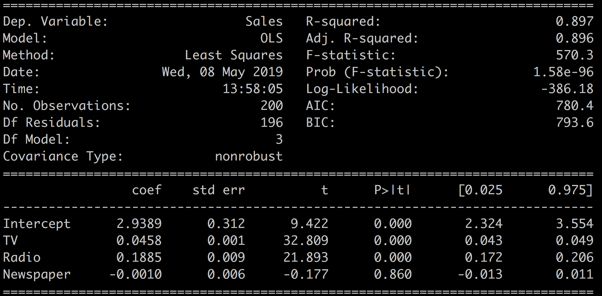
A couple of things stand out:

• R-squared = 0.897. Compare that with the R-squared = 0.612 that we had for the model Sales ~ TV in the previous chapter. Adding the two other variables increased R-squared significantly. This explains close to 90% of the sales variable with the new model! 

• Newspaper = -0.001. The Newspaper variable has a negative coefficient! :waw:
  This would indicate that the more you spend on newspaper ads, the less you sell. This really does not make sense.

Regression Coefficients With Multiple Predictors

In the context of multivariate linear regression, a coefficient tells you how much the input variable is expected to increase when that input variable increases by one, holding all the other input variables constant. For instance, if you increase the radio budget by $1,000, the coefficient 0.1885 tells you that, all other variables being constant, sales will increase by $188.5.

Interpret the Results

In the last chapter on univariate regression, we worked on some of the metrics available in the  results.summary(). In particular, we focused on:

• R-squared: a measure of the predictive power of the model.

• The predictor coefficient and associated p-value.

• The t-test,standard error, and the confidence interval.

Let's now look at some of the other metrics available in the results summary.

We have two new metrics to assess the quality of the model:

• Adj. R-squared: a version of R-squared that takes the complexity of the model into account.

• The F-statistic that tells you if your model is any better than a nothing model.

And three new metrics for model comparison:

• The log-likelihood: a measure of the probability of each sample given the model.

• AIC and its cousin BIC based on the number of samples and the log-likelihood.

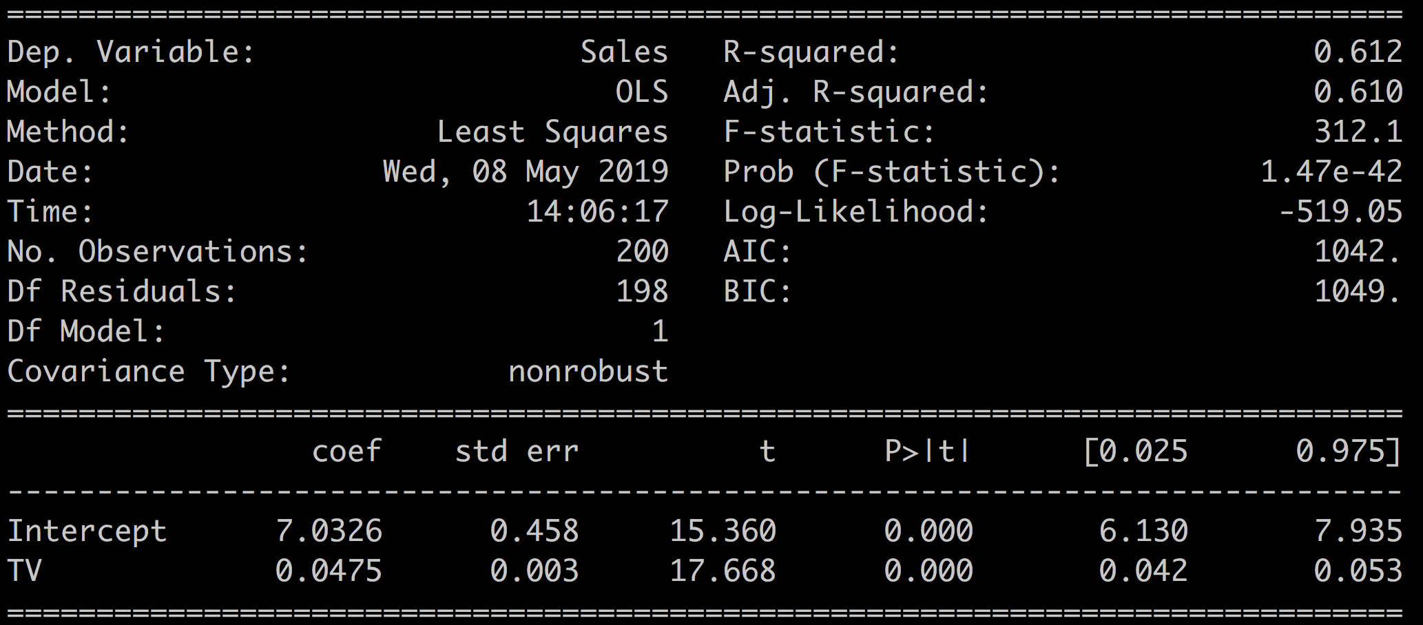
We use the model from the previous chapter to illustrate these multivariate model-comparison metrics: M1: Sales ~ TV versus M2: Sales versus TV + Radio + Newspaper.

The Sales ~ TV results are recalled here:

Adj. R-Squared

There's a well-known catch with linear regression.

Adding more and more input variables to your model almost always increases the R-squared value at the expense of complexity. As each new variable adds information to the model, its predictive power increases little by little with each extra predictor. R-squared increases a bit every time you add a predictor. However, after a certain point adding variables will only model the noise in the dataset instead of the true relationships between the predictors and the outcome.

For instance, you could build a model adding multiple variations of the original input variables          ($\$\backslash (log(TV)\backslash )\$$ , $\$\backslash (Radio^2\backslash )\$$ , $\$\backslash (\backslash frac\{1\}\{Newspaper\}\backslash )\$$, ...). Or you could add many new variables from secondary datasets, extra information about the students to the original school dataset, or tons of details related to the cars in the auto-mpg dataset. 

To balance this increase in R-squared and complexity of the model, you can look at the adj. R-squared. The adjusted R-squared is a modified version of R-squared that penalizes large numbers of predictors in the model. Adjusted R-squared only increases if adding a new variable improves the model more than would be expected by chance.

For most models, R-squared and adj. R-squared have very similar values.

In our case, adding the two other variables: radio and newspaper to the model, has improved the quality of our model since both R-squared and the adjusted R-squared have increased.

F-statistic and F-proba

The F-statistic tests the overall significance of the regression model by comparing the full model against a model where all of the regression coefficients are equal to zero, keeping only the intercept. It tells you if your model is better than nothing. 

The associated null hypothesis is defined as:

 $\$\backslash (H\_0\backslash )\$$ : The coefficients of the predictors are all equal to 0.

Which means that the predictors do not add any information to the outcome when compared to a model that just takes the intercept into account.

• The associated F-proba is the p-value for this null hypothesis. 

• The F-statistic can take any value superior to 1. 

• F = 1 means that the model is not better than a constant value.

In our case, we have for our two models:

Which shows that:

1. Both models are statistically significant and better than a simple constant model.

2. The multivariate model explains more of the outcome variable variance than the univariate model. 

Log-likelihood

The log-likelihood is a measure of the probability of seeing the data you have if that data was generated by your model.

In short:

• The log-likelihood is always a negative number because you are taking the log of probabilities whose values are by definition within [0,1].

• A better model leads to higher probabilities of observing the samples in your dataset and higher values of the log-likelihood.

• The higher the log-likelihood is, the better.

In our case:

Which shows that the multivariate model is better than the univariate one since -386.18 > -519.05.

Log-likelihood is an important concept which directly drives the calculation of the coefficients. You will see log-likelihood again at the end of Part 2.

AIC and BIC

Next, we look at AIC and BIC, which stand for Akaike information criterion (AIC), and Bayesian information criterion (BIC). Both metrics are used to compare models. There is no "good" value for them as they are both relative statistics.

AIC balances the complexity of the model (number of parameters) with its performance (log-likelihood). The number of parameters acts as a penalty term on the performance of the model (the log-likelihood). This is similar to the adjusted R-squared statistic, which also balances complexity with performance.

In other words:

• AIC estimates the relative amount of information present in the dataset which is lost by a model.

• The less information a model loses, the higher the quality of that model.

• The preferred model is the one with the minimum AIC value.

BIC is very similar to AIC. In BIC, the penalty term for the model complexity is more important, and also takes the number of samples into account.

Similar to AIC, the model with the lowest BIC is preferred.

In our case, we have:

This reflects that the multivariate model is better at modeling the data than the univariate model since it leads to lower AIC and BIC.

Cheat Sheet - Recap of the Metrics

You've seen quite a few ways to assess and compare the reliability and performance of your models. The following tables recapitulate what to look for when comparing models built on the same dataset.

Asses the Relevance of Your Model

To understand the quality of your model, look at these indicators:

Compare Models

For model selection, look at these indicators:

This wraps up our second tour of the different metrics of the results summary. We haven't looked at the bottom part of the summary that includes metrics like Omnibus, Skew, Durbin-Watson, and others. These are mostly used to assess the quality of the dataset and are explained in the next chapter.

Guided Exercise

In the following screencast, we study the difference between several models:

• The full multivariate model Sales ~ TV + Radio + Newspaper.

• The multivariate model without the Newspaper variable Sales ~ TV + Radio.

• And alternate model that mixes TV and Newspaper Sales ~ TV + Radio + TV*Newspaper.

Look at how these different models perform, and select the best one using the metrics of this chapter.

Summary

In this second chapter on linear regression, we worked on a multivariate model, and addressed the following items:

• Using formulas to define regression models.

• Definitions and interpretation of new metrics: Adjusted R-squared, F-statistic and F-proba, AIC and BIC.

• The impact of standardization of the variable on the regression results.

• The link between regression and correlation coefficients.

So far, we've applied linear regression to a few datasets without asking too many questions about the operation validity and the nature of the data. However, linear regression is not a generic method that can be blindly applied to any type of dataset. Some conditions need to be met! We will see this in the following chapter!

Go One Step Further: Frequently Asked Questions

Let's take a moment to address some frequently asked questions:

• What's the difference between regression and correlation coefficients?

• What's the impact of standardizing the data?

Regression Versus Correlation

Both regression and the correlation coefficients are a measure of the influence of the predictor on the outcome. However, they differ in the way they represent that influence.

In the univariate case, regression and correlation coefficients share the following properties:

• The regression coefficient is equal to Pearson's correlation coefficient.

• The square of Pearson's correlation coefficient is the same as the R-squared.

However, regression and correlation coefficients are different measures of the data. Here are a few differences:

• Correlation is symmetrical, while linear regression is not. Swapping the outcome with one of the predictor in multivariate regression will not give you the same coefficients.

• Linear regression can be used to make predictions, correlation coefficient cannot.

• Correlation works for nonlinear relations between variables, while linear regression works on linear relationships.

So correlation and regression are complementary, but intrinsically different ways of measuring the coupling between variables.

Standardizing Your Data

What's the impact of standardizing the data, and should you do it? That question often comes up in online forums. In short, this has no impact on the quality of the model, but it can help to interpret the coefficients.

The value of the regression coefficients depends on the average of the input variable. The higher the average of the variable, the lower its coefficient. The mean of the TV and radio budget variables is:

print(df[['TV','Radio']].mean())
TV 147.0425
Radio 23.2640

TV advertising is roughly six times as important as radio. The magnitude of coefficients of the linear regression reflect that disparity. The radio coefficient is roughly five times bigger than the TV coefficient

print(results.params)
Intercept 2.938889
TV 0.045765
Radio 0.188530
Newspaper -0.001037

Should we standardize the input variables to compensate for large differences in scale?

Standardizing the variables will change the value of the regression coefficients, but will not  influence the conclusions of the regression.

However, regression coefficients for standardized data cannot be interpreted as a relative measure of importance on the outcome variable. The deviation and mean of an input variable are not the only factors in determining the influence of a variable on the outcome.

To illustrate that point, let's standardize our data:

df_standardized = (df - df.mean()) / df.std()

Run a regression:

model_standardized = smf.ols(formula='Sales ~ TV + Radio + Newspaper', data=df_standardized)
results_standardized = model_standardized.fit()

Look at the results:

print(results_standardized.summary())

Which gives:

R-squared, F-statistics, t-test, and p-values have not been modified by the standardization of the variables. The values of the regression coefficients have changed and are easier to read, but less interpretable. In conclusion, for linear regression, there's no need to standardize your data except to make coefficients easier to read.