Design Effective Statistical Models to Understand Your Data

In the previous chapters, we've applied linear regression on the dataset without any concern for the reliability of the modeling methodology. However, linear regression is not a magic tool that works all the time on all datasets. Imagine fitting a linear model over a dataset like this one.

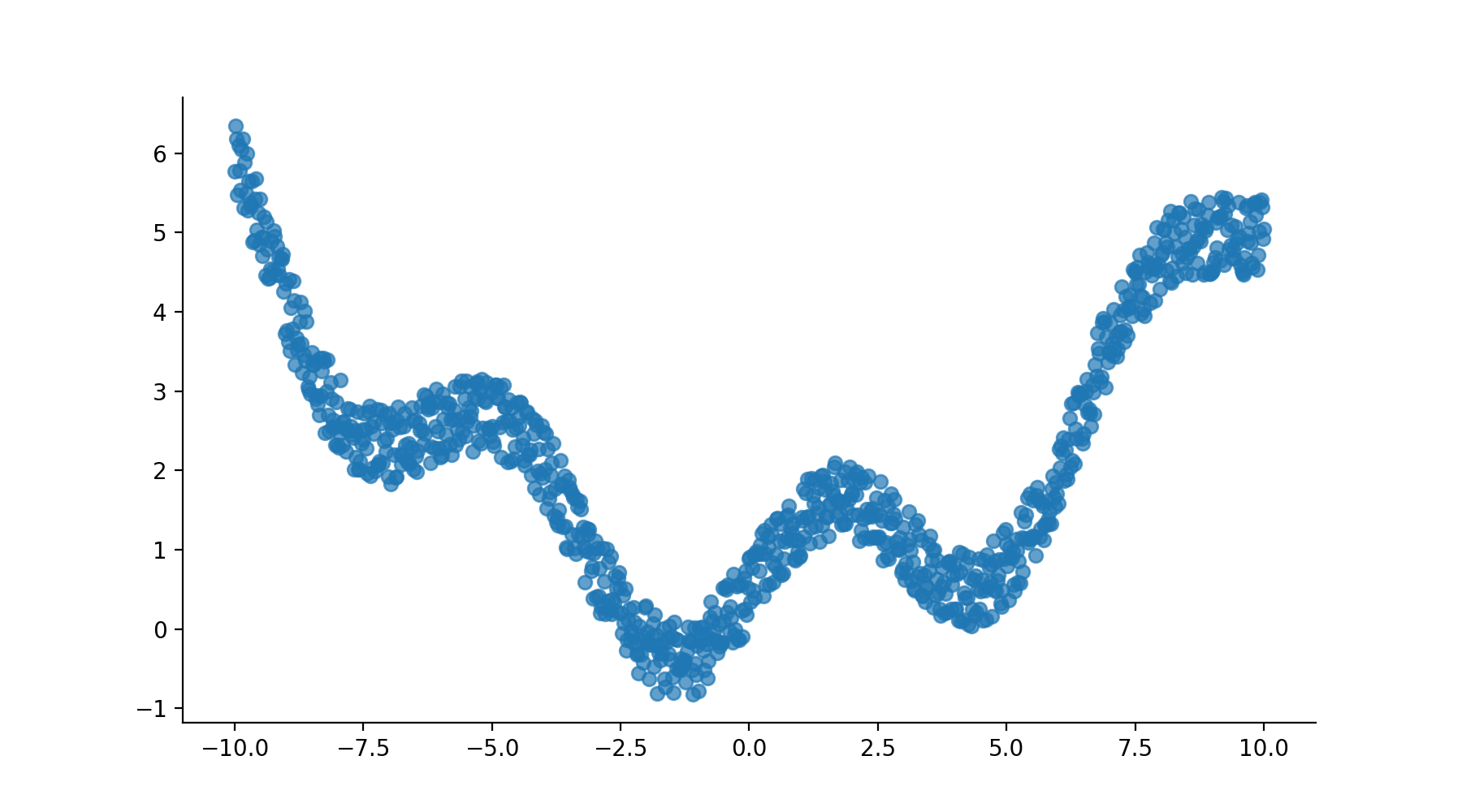
In fact, the data must verify five assumptions for linear regression to work:

Two conditions on the predictors and outcome:

• Linearity: the data has to be somewhat linear. 

• Collinearity: the predictors are not correlated.

And three conditions on the residuals of the regression:

• Autocorrelation: the residuals are not correlated to one another.

• Normality: the residuals must be normally distributed.

• Homoscedasticity: the variance of the residuals is stable (the inverse is called heteroscedasticity!)

Real-world data rarely plays nice, and most of the time, these assumptions are not fully met. In certain cases, this can have a significant impact on the results of the regression and skew its interpretation. Fortunately, there are ways to make the data more docile and regression-friendly.

In this chapter, we will go over each one of these  assumptions, investigate what happens when they are not met, and provide remedies. Let's start with the first assumption.

1) Linearity

The linear relationship assumption states that the relationship between the outcome and predictor variables has to be linear. This is a bit of a chicken and egg statement. Since you're using linear regression, you need the data to be linear so it can produce good results.

Testing for Nonlinearities With a Graph

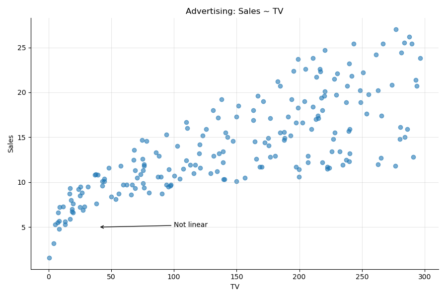
That said, the easiest way to test for linearity between each predictor and the outcome is to plot the predictor versus outcome scatter plots one by one.

In the advertising dataset, the scatter plot of the outcome sales versus the predictor TV shows a definite nonlinear relationship. As you can see in the following plot, the bottom left shows a distinct curve. The plot looks as if some smoke is erupting, and the wind is making it drift to the right.

Applying a Correction

To correct that nonlinearity, apply a nonlinear transformation to the variable of interest. The usual transformations are simple functions like log, sqrt, square, inverse, etc.
In our particular case, taking the square root of the TV variable will "redress" the graph, and display a more linear relationship: $\$\backslash (Sales\; \backslash sim\; \backslash sqrt\{TV\}\backslash )\$$

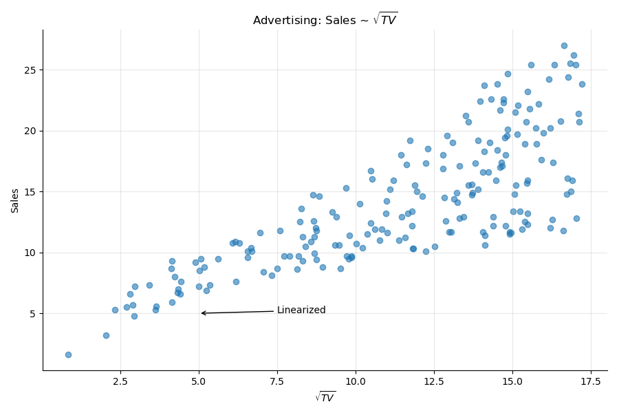
Since we modified the predictor $\$\backslash (TV\backslash )\$$ into $\$\backslash (\backslash sqrt\{TV\}\backslash )\$$ , we can compare the two models. The model $\$\backslash (Sales\; \backslash sim\; \backslash sqrt\{TV\}\backslash )\$$ shows slightly better results than the original $\$\backslash (Sales\; \backslash sim\; TV\backslash )\$$ model.

Testing for Nonlinearities With Another Graph

Another way to detect nonlinearities in the dataset is to plot the residuals versus the fitted values of the results, as you saw in Chapter 2.1. Plots that display a distinct pattern hint at the presence of nonlinearities. For illustration, here are the residuals versus fitted values for the model  mpg ~ HorsePower  from the auto-mpg dataset introduced in Part 1. You can see a distinct quadratic pattern illustrated by the orange interpolation line:

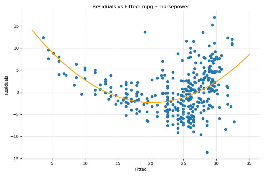
In that case, a model that takes into account the square of horse power $\$\backslash (mpg\; \backslash sim\; HorsePower^2\backslash )\$$  would deal with this nonlinearity.

2) Collinearity

The second assumption on the data is called collinearity, which means  that several of the predictors are (co)related to one another:

• Several predictors are highly correlated.

• Some hidden variable may be causing the correlation.

Predictor collinearity negatively impacts the coefficients of the model.

Demo

Let's go back to the advertising dataset and look at the correlation of our predictors.

df = pd.read_csv('advertising.csv')
df.corr()

This outputs:

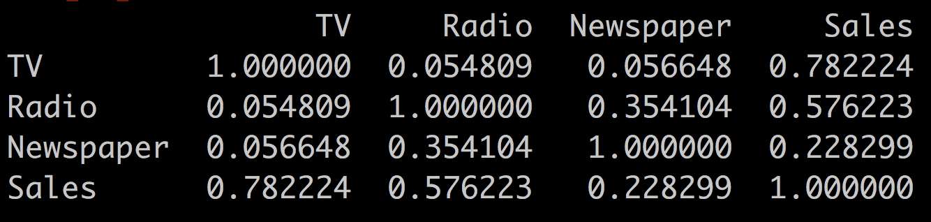
You see that radio and newspaper are correlated to each other (r = 0.35), while newspaper and TV are not (r = 0.05). Let's see the difference this makes when we compare the two models:

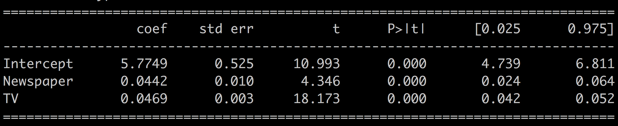
• Uncorrelated predictors:  Sales ~ TV + Newspaper

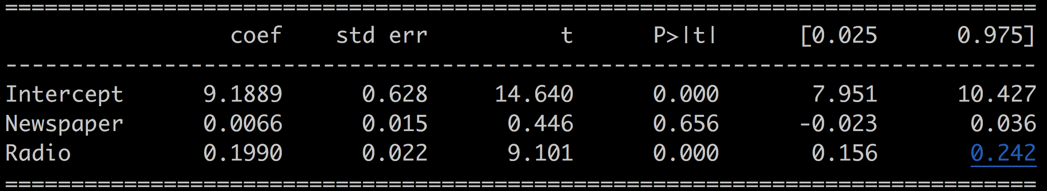
• Correlated predictors: Sales ~ Radio + Newspaper

For the first model, where the predictors are not correlated, we have:

And for the second model where the predictors are correlated, we have:

Interpretation

The p-values for the newspaper coefficient are well below 0.05 for the first model and well above 0.05 for the second. In the first uncorrelated case, the predictors are independent of one another, and the model is reliable; whereas in the second case, there's some hidden factor common to the predictors, and the regression is not reliable.

Detecting Multicollinearity

There are multiple ways to detect multicollinearity among the predictors.

Correlation Matrix

The first way to detect multicollinearity is to look at the correlation matrix of the predictors and weed out all predictors too correlated with one another.

Variance Inflation Factor (VIF)

However, not all collinearity problems can be detected by inspecting the correlation matrix. Collinearity can exist between two or more variables, even if no pair shows a particularly strong correlation. This situation is called multicollinearity.

Instead of inspecting the correlation matrix, a better way to assess multicollinearity is to compute the variance inflation factor (VIF), which measures the degree of multicollinearity introduced by adding a predictor.

VIF is available from the statsmodels library:

from statsmodels.stats.outliers_influence import variance_inflation_factor as vif

The VIF function takes the list of predictors and the index as input of the predictor for which you want to calculate the VIF.

For example, in the regression: Sales ~ TV + Radio + Newspaper, calculate the VIF for TV with:

# VIF for TV
vif(df[['TV', 'Radio', 'Newspaper']].values, 0)
> 2.487

And the VIF for radio and newspaper respectively with:

# VIF for Radio
vif(df[['TV', 'Radio', 'Newspaper']].values, 1)
> 3.285
# VIF for Newspaper
vif(df[['TV', 'Radio', 'Newspaper']].values, 2)
> 3.055

As a rule of thumb, a VIF value that exceeds five indicates a problematic amount of multicollinearity. In our case, none of the three predictors is causing too much collinearity.

Condition Number

Finally, the condition number (Cond. No.) displayed in the lower half of the results summary is also a direct measure of multicollinearity. Smaller values (<20) indicate less multicollinearity.

Solution

In the presence of strong multicollinearity, the solution is to drop the predictor most correlated with the others from the model. In our case, that would be the newspaper variable since radio and TV are not particularly correlated with one another.

3) Autocorrelation of Residuals

This second assumption dictates that the residuals of a linear regression model should not be correlated to one another. In other terms, the error $\$\backslash (e\_i\; =\; y\_i\; -\backslash hat\{y\_i\}\backslash )\$$ related to the sample $\$\backslash (i\backslash )\$$ should be independent from the  error $\$\backslash (e\_\{i-1\}\backslash )\$$ related to the sample $\$\backslash (i-1\backslash )\$$ .

How do we test that the residuals are truly uncorrelated?

If you recall the results summary of the linear regression, in the lower part of the summary, there was a line for the Durbin-Watson test. The Durbin-Watson statistic is a direct test of the correlation of the residuals. It takes a value from 0 to 4, where:

• 2 means no autocorrelation.

• 0 to 2 means positive autocorrelation.

• 2 to 4 means negative autocorrelation.

• As a rule of thumb, values in the range of 1.5 to 2.5 are relatively normal.

The Durbin-Watson statistic for the Sales ~ TV + Radio + Newspaper model is:

• Durbin-Watson: 2.084

Showing that the residuals are not correlated.

4) Normality of the Residuals

You already saw this in the previous chapter when checking the quality of the model by looking at the probability distribution of the residuals. When the model catches all the information in the data, the residuals should follow a normal distribution.

Checking the Distribution

You've  already seen several ways to assess that property of the residuals:

1. Using a Kolmogorov-Smirnov test for goodness of fit.

2. Drawing the QQ plot. 

3. Plot the histogram of the residuals and compare it with the histogram of a normal distribution.

Jarque-Bera Statistic

A fourth way is in the results summary using the  Jarque-Bera statistic.

This statistic tests the null hypothesis that the residuals are normally distributed. This means that if the p-value is below the 0.05 threshold, you can reject the null hypothesis, and your residuals are not normally distributed. It does not mean that if the p-value is above 0.05, you can conclude that the residuals are normally distributed, just that you cannot say with certainty that they are not normally distributed.  Don't you just love hypothesis testing? o_O

The remaining assumption has a terrible name: heteroskedasticity! :diable: It relates to the variance of the residuals.

5) Variance of Residuals

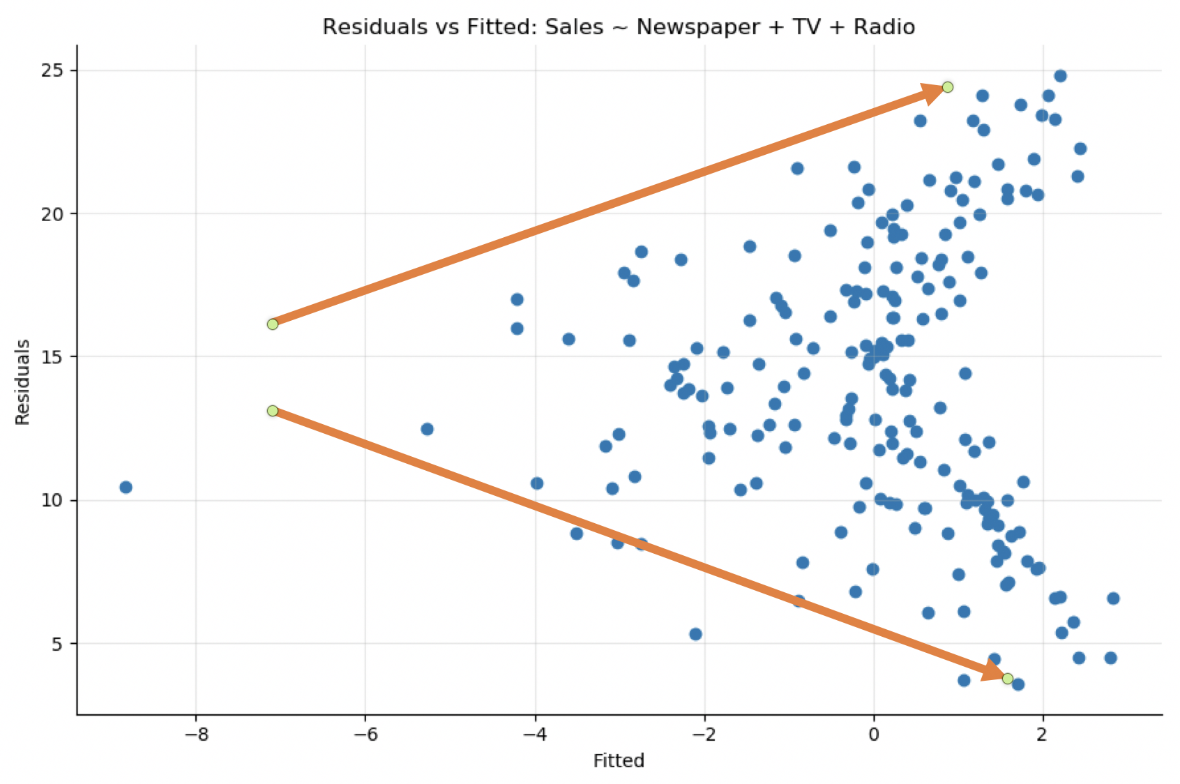
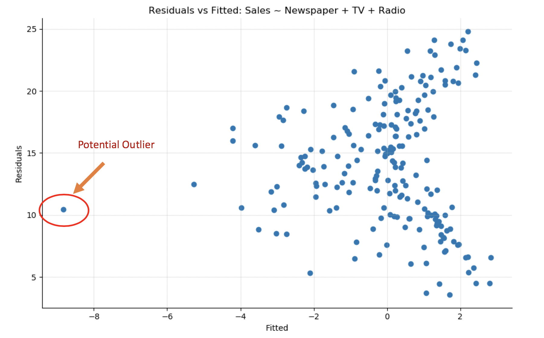
The heteroskedasticity assumption means that the variance of the residuals has to be constant for the regression to be reliable. You can detect it by plotting the residuals versus the fitted values. The variance of the residuals should not increase or decrease as the fitted values increases.

Looking at the residuals versus fitted plot of the model  Sales ~ TV + Radio + Newspaper, you see that the variance of the residuals is not constant. There's a definite funnel-shaped pattern. As the fitted values increases, so does the range of residual values:

Solution

The solution is to apply a concave function such as log or sqrt to the outcome variable.

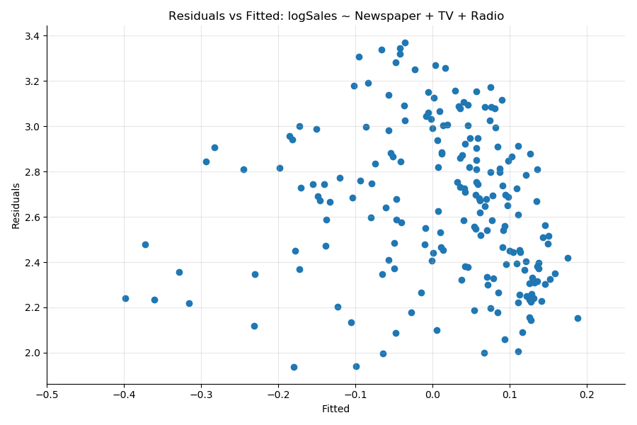
For example, if we create the new variable as the log of sales:

df['logSales'] = np.log(df.Sales + 1)

Build a model with that new target variable:

results = smf.ols('logSales ~ Newspaper + TV + Radio', data = df).fit()

You see that the heteroskedasticity (the funnel pattern in the previous plot) has been greatly reduced:

The statistical test to measure heteroskedasticity is the ‎Breusch–Pagan test available in the statsmodel library.

Cheat Sheet: The Five Main Assumptions and How to Test Them

Solutions

Remove Outliers

Outliers are extreme values taken by one of your variables. There is no strict definition of what constitutes one; it depends on your dataset and modeling approach.

Once you've identified the outliers in your data, you have a choice of either discarding the sample and removing it from the dataset or replacing it with a more adequate value such as the mean of all the values or some specific value that makes sense.

You can find a potential outlier in the auto-mpg dataset by looking at the residuals versus fitted. The point in the lower-left of the plot is probably an outlier. It also appears on other plots (Sales vs. TV). Removing it may improve the model. The question, however, is if that sample is an anomaly or representative of the dataset.

Transform Variables

Transforming a variable changes the shape of its distribution and often helps in:

• Dealing with nonlinearities.

• Making the variable distribution closer to a normal distribution.

The go-to method to make a distribution more normal is to take the log of the variable $\$\backslash (log(X+1)\backslash )\$$ . Other ways to transform nonlinear patterns include powers of the variable  $\$\backslash (X^2,\; X^3,\; \backslash sqrt\{(X)\},\; \backslash cdots\backslash )\$$ , inverse  $\$\backslash (\backslash frac\{1\}\{X\}\backslash )\$$ , and so forth. Although taking the log is often a good strategy, finding the right transformation can be full of trials and errors.

Summary

Linear and logistic regression is far from a black-box model that you can simply apply to any dataset to make predictions and analyze the relationships between your variables. As you've seen in this chapter, five main assumptions need to be respected to be confident with your models:

• Linearity between the predictors and the outcome.

• The residuals must not be correlated. 

• Absence of multicollinearity between the predictors.

• The residuals should be normally distributed. 

• The residuals variance should be constant. 

Potential solutions include transforming the variables or simply removing a predictor from the model.