Build and Interpret a Logistic Regression Model
So far, we've exclusively worked with continuous outcome variables, i.e., that could take any value positive or negative, as little or large as possible. However, there are many cases in real life where you may want to model a categorical outcome (A variable that can take only a few specific values.) instead of a continuous one. Modeling a categorical outcome variable is called classification. And the classification method is called logistic regression.
Why Linear Regression Doesn't Work
Linear regression does not work for classification. Let's look at an example to see why.
You want to predict categories that are not inherently ordered, for instance, an animal. If you used linear regression and set arbitrary thresholds on the outcome variable:
such that:
y < -5 then cat
-5 < y < 5 then dog
y > 5 then rabbit
You would introduce an artificial order between the categories that is not present in the first place. Why would cat < dog < rabbit make more sense than dog < rabbit < cat?
Linear regression is not the right tool to model categorical outcomes.
That does not mean everything is lost. We simply need to modify linear regression to handle classification models. This modeling approach is called logistic regression, and you will soon see why it is called logistic regression and not logistic classification.
From Linear Regression to Logistic Regression
In short, logistic regression is an evolution of linear regression where you force the values of the outcome variable to be bound between 0 and 1. The bounded values are then interpreted as the probability of belonging to one of the categories in which we're interested.
How can you transform the results of a linear regression to predict a binary category?
You first need to make sure that the outcome is contained in the interval so it can be interpreted as a probability .
To force the outcome to be between 0 and 1, apply the logistic function.
Then set an arbitrary threshold, for instance 0.5, and decide that if . The output is classified as the 1st category and if p > 0.5 as the 2nd one.
To recap:
is the standard linear regression
and
is a probability because it belongs to
if then classify the sample as category 1 else classify as category 2
As you can see, we are using linear regression and adapting it to predict a binary variable. This is why logistic regression is called a regression:
Logistic comes from the use of the logistic function.
Regression comes from the use of linear regression.
Logistic Function
So what is that logistic function about?
The logistic function also called sigmoid function, or S curve, is a function that takes any real value and outputs a number contained within the interval
The graph of the logistic function is:
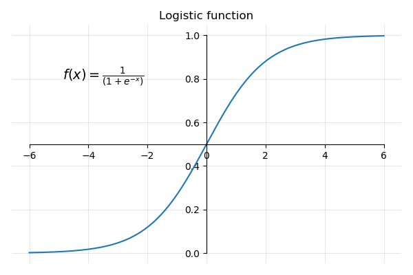
As you can see:
For very large positive values of x, and
For very large negative values of x , becomes very large and the fraction
So the output of the logistic function is always between 0 and 1 for all values of x.
Now that you get the gist of how to modify linear regression for classification tasks, let's apply logistic regression to some real data. As you will see, most of what you learned about linear regression is still relevant.
Classification of Credit Default
A typical use of binary classification is to detect whether or not a person will default on her or his credit card payments. Fortunately, there is an open-source Credit Default dataset.
That dataset has the following predictors:
Continuous variables: balance, and income.
Binary variable: student which indicates if the person is a student or not.
The outcome variable: default which indicates whether the person defaulted on his/her credit loan. Default is a binary variable that takes the values yes and no with the following counts:
No 500
Yes 333
Let's load the dataset:
import pandas as pd
df = pd.read_csv('credit_default.csv')
print(df.head())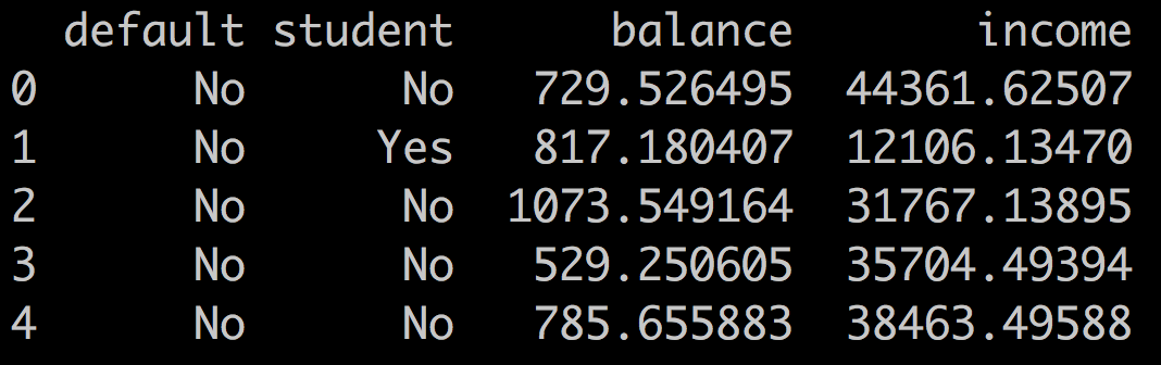
Logistic Regression With Statsmodel.logit()
Let's build a logistic regression using the logit method in statsmodel. The logit method works the same as the ols method we used for linear regression by taking a regression formula as input. The results are very similar and the metrics are the same. Some have changed name, but can be interpreted in the same way.
Before we build the model, we need to transform the values of our default variable from text (yes/no) to numbers (0/1) because statsmodel only works on numerical values. For that, write:
df.loc[df.default == 'No', 'default' ] = 0
df.loc[df.default == 'Yes', 'default' ] = 1We only consider the continuous predictors: income and balance. Similarly to the multivariate linear regression we built in the last chapter, we can define the model and fit it with:
import statsmodels.formula.api as smf
model = smf.logit('default ~ income + balance', data = df)
results = model.fit()
print(results.summary())
Which outputs:
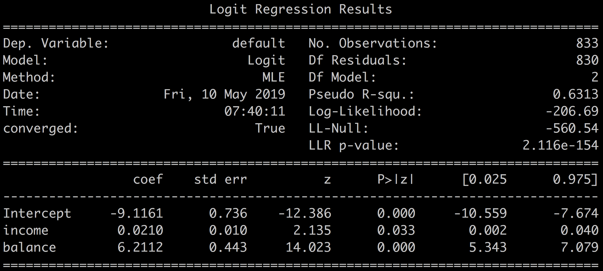
You should recognize several metrics that are common to both the logistic and the linear regression results summary:
Coefficients, p-values, standard error, and confidence intervals.
Log-likelihood.
Some metrics have different names:
Pseudo R-squ. is a substitute for R-squared. It also measures the amount of outcome variable variance, which is explained by the model. Pseudo R-squared can be interpreted in the same way as R-squared; the higher the better, with a maximum of 1.
LL-null and LLR p-value are equivalent to the F-statistic and F-proba of linear regression, and are interpreted in the same manner for comparing models.
The higher the value for LL-null the better. Low values for LLR p-value (<0.05) mean you can reject the null hypothesis that the model based on the intercept (all coefficients = 0) is better than the full model. Hence, our model is relevant.The z-statistic plays the same role as the t-statistic in the linear regression output and equals the coefficient divided by its standard error. The lower, the better.
Model Assessment
Looking at these results, how good is our classification model?
Balance and intercept p-values are below 0.05. You can trust the balance and intercept coefficients. This is reinforced by the relatively low values for associated standard errors.
The reliability of the income coefficient is less straightforward with a p-value of 0.033; very close to 0.05.
results.pvalues
Intercept 3.120011e-35
income 0.033
balance 1.122455e-44
Pseudo R-squared = 0.6313. 63% of the default variable variance is explained by our model. Not a fantastic score, though.
You can also conclude that balance seems to be a better predictor of default than income as the coefficient, and the z-value is lower for income than it is for balance.
To assess the classification performance of the model, there are two things you can look at:
The output of the logit function.
The predicted class for all the samples.
Let's take a look!
The Histogram of Probabilities
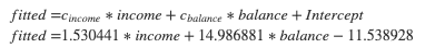
The results.fittedvalues correspond to the results of the linear regression:
To obtain the probabilities, apply the logistic function to the fitted values:
proba = 1 / (1 + np.exp( - results.fittedvalues ))The histogram of the probabilities offers a very good visual assessment of the model quality.
A good model will clearly separate the two classes, and for most samples, the probabilities will be concentrated around 0 or around 1.
A less performing model will have a tendency to hesitate and produce probabilities centered around the threshold value 0.5.
The histogram of probabilities for our model gives:
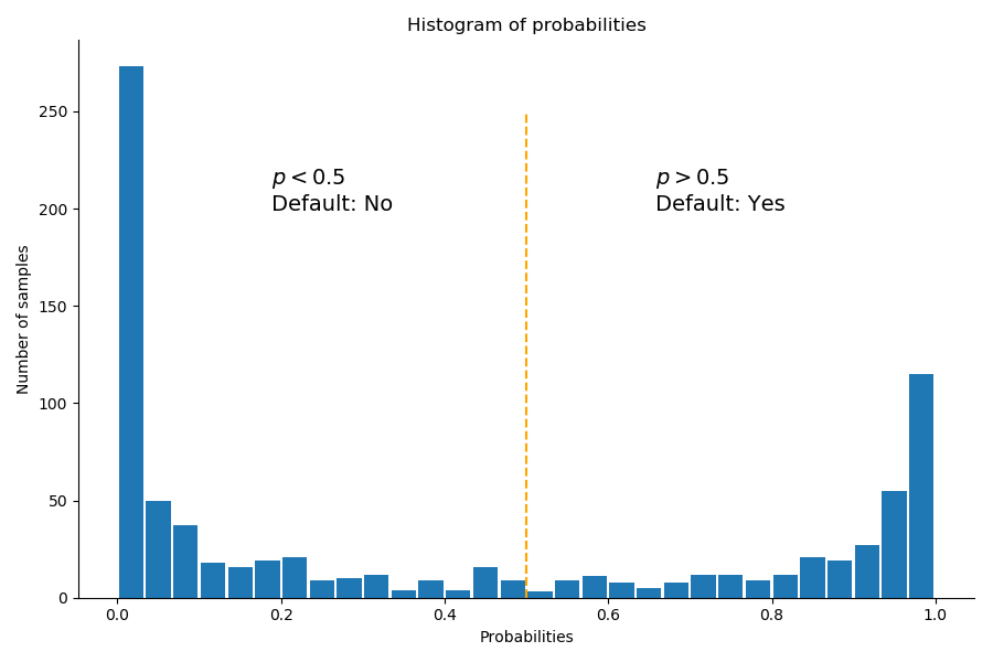
We have two distinct peaks near 0, and near 1. The model is almost always certain that a sample belongs to the non default (No, ) , or the default (Yes - ) category.
The samples closer to middle of the plot ( ) are less obviously classified in one class or the other.
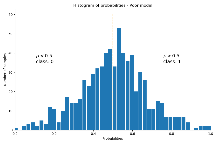
For comparison purposes, the following graph shows the probability output of a classification model on a different dataset that does not discriminate well between the classes. Notice that the bulk of samples have probabilities in the middle of the graph close to 0.5. That model hesitates in its classification.
The Predicted Class
A more straightforward way to obtain the class probabilities is to use the predict function as such:
yhat = results.predict(df[['income', 'balance']])That is equal to the probabilities we calculated with:
Obtaining the predicted classes from the probabilities comes down to setting a threshold at 0.5 and running this code:
threshold = 0.5
# transforms the list of booleans into an int with 1 = True, 0 = False
predicted_class = (yhat > threshold).astype(int)
print(predicted_class)
> [1,1,1,1...,0,0,0]
You can further investigate the quality of the model based on the predicted classes with the confusion matrix.
Confusion Matrix
In essence, classification is about putting the right samples in the right class. Non-default in the 0 class and default in the 1 class. Digging deeper, we want to know how many yes's and no's were correctly identified. In other words:
How many samples were correctly classified: true positives and true negatives.
How many samples incorrectly classified by the model.
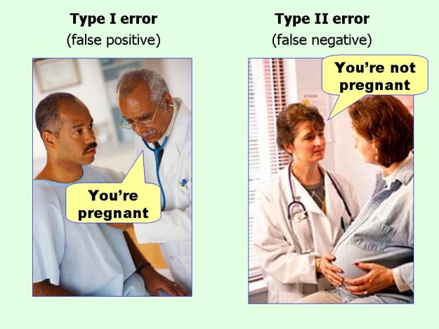
More precisely:False positives: how many default (1) samples are mistakenly classified as non-default (0).
False negatives: how many non-default (0) samples are mistakenly classified as default (1).
Depending on your context, you may want to focus on one or the other type of error.
For instance, in intrusion detection systems, since it's better to be falsely alerted than to miss a real intrusion, you will focus on minimizing false negatives at the expense of false positives.
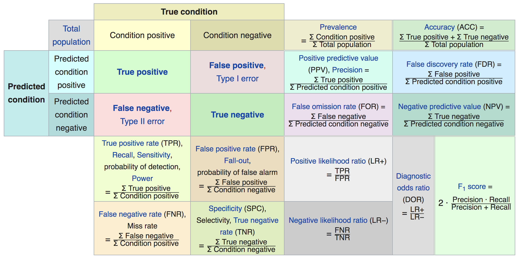
A confusion matrix is a table that summarizes these four metrics:
| Predicted 1 | Predicted 0 |
Actual 1 | True positives | False negatives |
Actual 0 | False positives | True negatives |
The confusion matrix for our model can be obtained with pred_table():
results.pred_table()Which gives:
| Predicted Default | Predicted Non-Default |
Actual Default | 286 | 47 |
Actual Non-Default | 40 | 460 |
Out of of 333 default samples:
286 were correctly predicted as default by our model (true positives).
47 were wrongly predicted as non-default by our model (false negatives).
And out of 500 non-default samples:
460 were correctly predicted as non-default by our model (true negatives).
40 were wrongly predicted as default by our model (false positives).
Interpreting Logistic Regression Coefficients
Contrary to the coefficients in linear regression, you cannot directly interpret the logistic coefficients by saying that if you increase the income by $1000 (the unit), the chance of defaulting is increased by 0.021% (income coefficient = 0.021).
For that, you need to exponentiate the coefficients:
np.exp(results.params)
Intercept 0.000110
income 1.021179
balance 498.308810Summary
Why is logistic regression, which is a classification method, called regression anyway?
Well, as you've seen in this chapter, logistic regression is based on:
Linear regression.
The logistic function that transforms the outcome of the linear regression into a classification probability.
Hence the name logistic regression.
In this chapter, we worked on the following elements:
The definition of, and approach to, logistic regression.
Interpreting the metrics of logistic regression: coefficients, z-test, pseudo R-squared.
Interpreting the coefficients as odds.
So far, all our predictors have been continuous variables. But nothing prevents you from having categorical variables as predictors - and this is what the next chapter is about!
One Step Further: Exponentiate the Coefficients
Mathematically speaking, the probability is given by:
The quantity is called the odds:
It can take on any value between 0 and ∞.
Values of the odds close to 0 and ∞ respectively, indicate very low and very high probabilities of default. Odds are preferred in some contexts (horse races for instance) as they lead to more realistic interpretations:
The odds of an event is the probability of that event divided by its complement:
Some examples:
For an event with probability 0.75, the odds are: . This means that the event is three times as likely to occur than not.
One in five people (p = 0.2) with an odds of 1/4 (0.25) will default, since p(X) = 0.2 implies odds of 0.2 / (1-0.2) = 1/4.
Likewise, on average, nine out of every ten people with odds of nine will default, since p(X) = 0.9 implies an odds of 0.9/ (1-0.9) = 9.
Go Even Further: Multinomial Regression
To wrap up this chapter on classification, let's wade into multinomial classification, where the outcome variable can take more than two classes.
There are two common ways to handle multinomial classification. In both cases, the idea is to come back to a binary classification:
One-vs-One
Let's say you have three categories: dogs, cats, and rabbits. In the one-vs-one strategy, you would train a model for each of the binary permutations:
M1: rabbits vs. dogs.
M2: cats vs. rabbits.
M3: dogs vs. cats.
At prediction time, the probability of a sample is the average probability over the two models for that sample.
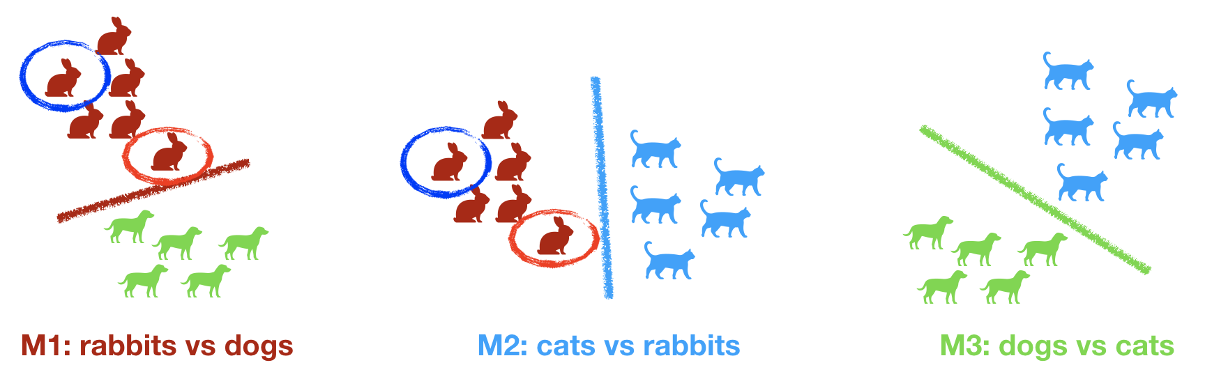
Consider the rabbit circled in blue. Visually, you can guess that that sample will have a strong probability of being classified as a rabbit with both M1 and M2. Its overall probability of being classified as a rabbit is the average of the probabilities given by M1 and M2.
On the contrary, the rabbit circled in red is closer to dogs and cats, and its probability under M1 and M2 would be closer to 0.5. The overall probability of that sample being a rabbit would be lower than for the rabbit circled in blue.
For N categories, this approach will have you build N(N-1) / 2 models, which can become time- consuming and complex for large number of categories.
One-vs-Rest
This approach is more sequential.
You arbitrarily pick one class, let's say rabbits, and train your model to distinguish between rabbits and all the other categories (cats and dogs).
You put aside all the samples that are identified as rabbits, and build a second binary model on the remaining sample that identifies dogs versus cats.
You end up building two models:
M1: rabbits vs. non-rabbits.
M2: remove identified rabbits, build a dog vs. cat model.
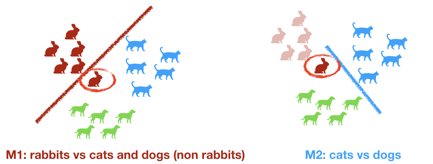
You usually pick the first category that is easiest to separate from the rest.
