Handle Categorical Predictors
At this point in the course, you can create linear and logistic regression models to work with continuous and categorical outcome variables. However, you have only worked with predictors that were continuous variables. It stands to reason that you can use categorical variables as predictors in a regression model.
The first way to exploit a categorical predictor is to add it to the regression model. If there are more than two categories, you need to break down the variable into multiple binary ones.
The other approach called ANOVA stands for Analysis of Variance. This method was formerly introduced in Fisher's 1925 classic book Statistical Methods for Research Workers. ANOVA is used to analyze the differences in the mean of groups of samples with respect to categories. It is a way to extend the t-test (remember Chapter 1.4 on hypothesis testing) to multiple groups and categories.
In this chapter, you will learn about:
How to add categorical values in a regression model:
With one hot encoding
Using formulas
Using binary encoding when the variable has way too many categories.
The ancient and respected techniques of ANOVA.
Throughout the chapter, we will work on the auto-mpg dataset to demonstrate how to handle categorical variables.
Let's get to it!
The Dataset
The dataset has four continuous variables and four categorical ones: cylinders, year, origin, and name. Cylinders and year are ordered, and can be used directly in the regression model. We are interested in the non-ordinal categorical variables:
The origin.
The name of the car.
Therefore, the origin variable is just a categorical variable with three values American, European, and Japanese.
American: 245 cars
Japanese: 79 cars
European: 68 cars
The other categorical variable available is the name. However, we have 301 different names for 392 samples. Instead of considering the name of the car as our categorical variable, we'll extract the brand of the car, which happens to be the first word in the name field.
For that, you use:
df['brand'] = df.name.apply(lambda d : d.split(' ')[0])Let's first consider the univariate model mpg ~ origin and use the origin variable as a predictor:
results = smf.ols('mpg ~ origin', data = df).fit()
results.summary()
Which outputs:
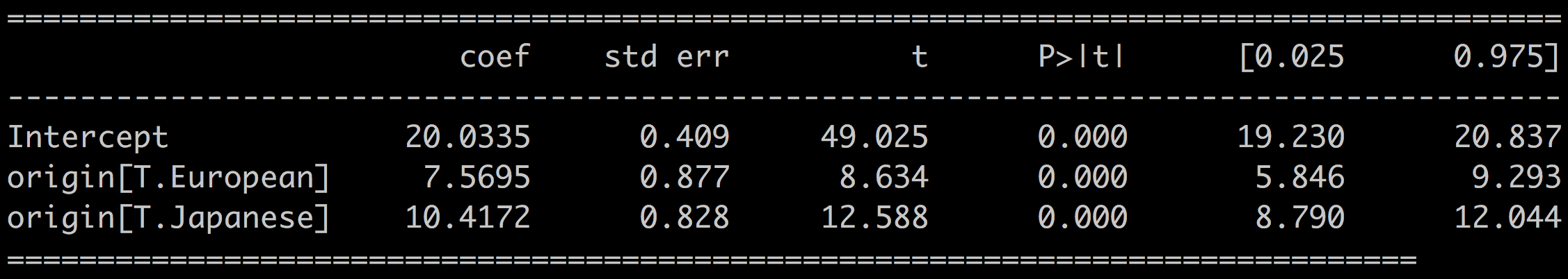
A couple of things stands out:
The stastmodel library has automatically handled the categorical feature by creating two variables: origin[T.European] and origin[T.Japanese].
We have three original categories, but only two of them show up in the results.
Dummy Encoding
What the library did is called dummy encoding, or one-hot encoding. Dummy encoding encodes a k-level categorical variable into k-1 binary variables. In our example, the variables origin[T.European] and origin[T.Japanese] are binary variables, which represent:
origin[T.European]: The car is from Europe: True/False
origin[T.Japanese]: The car is from Japan: True/False
You can always deduct that a car is American if it's not either European or Japanese, and there's no need to include the third binary variable origin[T.American]. Doing so would introduce high level of collinearity in the model and degrade its reliability.
Dummy Encoding With Pandas
Instead of letting statsmodel handle the encoding of the categorical variable, we could have done this dummy encoding manually with the pandas.get_dummies() function:
pd.get_dummies(df.origin).head()It outputs three variables: American, Japanese, and European that can be merge into the original DataFrame:
df = df.merge(pd.get_dummies(df.origin), left_index=True, right_index= True )
print(df.head())
The model:
results = smf.ols('mpg ~ Japanese + European', data = df).fit()The exact same results as before with the mpg ~ origin model.
Interpreting the Coefficients
Let's calculate the mean of the mpg variable by origin. With pandas, it's a one-liner:
df[['mpg','origin']].groupby(by = 'origin').mean().reset_index()Which returns:

Compare these values to the coefficients of the mpg ~ origin model:

You can notice that:
The Intercept is the mean of mpg for American cars (the left-out binary variable)TheThe
In a univariate regression with a categorical predictor:
The Intercept is the mean of the outcome for the left-out category:
.
The coefficients of the other categories are the means of the outcome for that category minus the intercept:
Which is pretty sweet! :soleil:
Now to a more complex case with the brand variable, which has 37 different categories.
Handling a Variable With Many Categories
With only three categories, the origin variable was easy to handle. On the other hand, the brand variable has no less than 37 values unequally represented (48 Ford, 3 Renault, and 1 Nissan).
If you use the brand variable to build the model mpg ~ brand, that will mean:
Having 36 predictors in the model, making it difficult to interpret.
Many unreliable coefficients for brands with few samples.
Dummy encoding does not scale for variables with large numbers of categories. There are several ways to solve that problem. Here are two simple and efficient ones:
Regroup all the categories with low representation into an other category.
Use binary encoding.
We will illustrate these two methods on the auto-mpg dataset.
Aggregating Rare Categories
Let's limit ourselves to American cars to make things more readable.
df = df[df.origin =='American']We have 15 brands; 5 of them with less than 5 samples each:
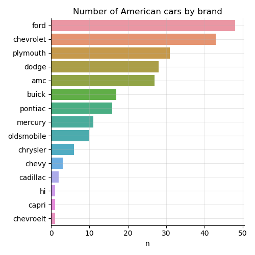
The simplest thing to do is group all the rare categories, such as those with less than 10 samples, into one catch-all other category.
df[df.brand.isin(['chrysler','chevy', 'cadillac', 'chevroelt', 'capri', 'hi']), 'brand'] = 'other'Then we have a much more even repartition of brands:
Ford 48
Chevrolet 43
Plymouth 31
Dodge 28
Amc 27
Buick 17
Pontiac 16
Other 14
Mercury 11
Oldsmobile 10
Here are the results for the model mpg ~ brand for American Cars:
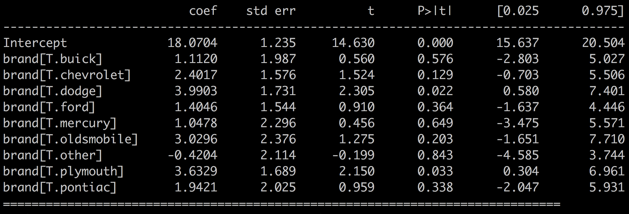
With:
R-squared = 0.058
F-statistic of 1.004
p-values > 0.05
You can safely conclude that the brand variable is not a good predictor of the fuel consumption for American cars.
Binary Encoding
Dummy encoding is simple to implement, but does not scale to many categorical values.
An alternative to dummy encoding is binary encoding. The idea is to transform the category into ordered numbers (1,2,3, ...,99,100,101, etc.) and then to convert that number into a binary representation (10010). Once you have the binary encoded version of the category, use each digit as a separate variable in the model.
On the plus side, binary encoding greatly reduces the number of new variables needed to represent the original categorical variable avoiding the curse of dimensions mentioned before.
On the down side, you can no longer interpret the influence of a category on the outcome, since all the categories are jumbled together.
Use binary encoding for building predictive models rather than the interpretability of the model.
Let's see how you apply that to the brand variable. This time, considering all the cars in the dataset, not just the American ones. There are 37 different brands.
In Python, binary encoding uses the category_encoders package:
import category_encoders as ce
# define the encoder
encoder = ce.BinaryEncoder(cols=['brand'])
df = encoder.fit_transform(df)
This will create six new variables brand_0, brand_1 to brand_5 directly into the DataFrame and drop the original variable brand.
Now we can define the new model mpg ~ brand_0 + brand_1 + brand_2 + brand_3 + brand_4 + brand_5 and we get R-squared = 0.270.
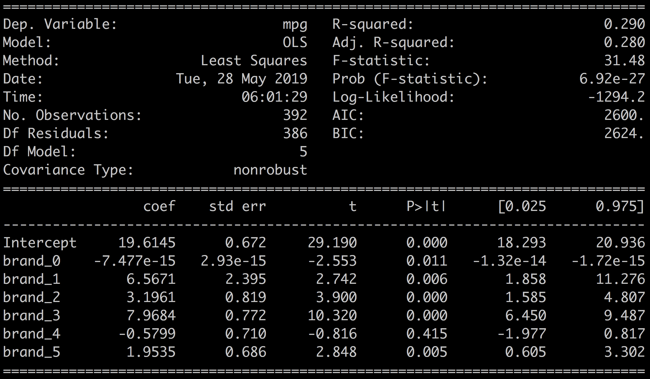
This is a decent model, but we have lost all possibility of interpreting the coefficients for the predictors brand_0, brand_1, ..., brand_5.
ANOVA
Let's switch gears and consider the much-respected ANOVA, or Analysis of Variance.
While working on the origin categorical variable, you've seen the coefficients related to the different categories in a univariate regression correspond to the mean or difference of means of the outcome for the different groups. In this scenario, groups are a subset of samples that belong to a certain category.
When the categorical variable takes only two values (binary), you can use the t-test to verify the statistical significance of the mean across the two categories. That's what we did in the previous exercise on hypothesis testing to analyze the difference in height between school girls and boys.
ANOVA is an extension of the t-test where the categorical variable takes more than two categories. ANOVA tells you if the differences in the variance between each group are statistically significant when compared to the differences within each group.
One-way ANOVA considers only one categorical factor (brand or origin), while two-way ANOVA considers two factors (brand and origin). In the framework, predictors are often called factors, and each category/group within a predictor is called a level.
We will only work with one-way ANOVA in this chapter and illustrate the method on the mpg vs. origin variables to establish if the origin of the car has a significant impact on the fuel consumption (on average).
One-Way Anova
The null hypothesis of ANOVA is:
H0: No difference between the means in the different categories.
The alternative hypothesis is:
Ha: There is a difference between the means in the different categories.
However, you don't know what the difference is or which group makes a difference.
In statsmodel, ANOVA is built on top of the results of the linear regression.
results = smf.ols('mpg ~ C(origin)', data=df).fit()
results.summary()
Then you apply the anova_lm function to the linear regression results as such:
aov_table = sm.stats.anova_lm(results)
print(aov_table)
You get the the following table:
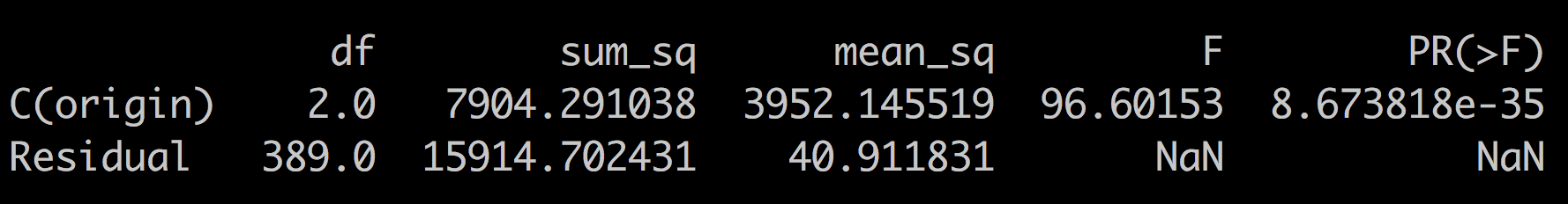
The important thing to focus on is the F-statistic and its p-value PR(>F).
If the null hypothesis is true (no difference in means between the categories), you expect F to have a value close to 1.0 most of the time. A large F, like the one we observe here, means that the observed variation between the different categories is not happening by chance.
Therefore, we can be certain that the fuel consumption mpg is different with American, Japanese, or European cars.
This does not tell us what category performs best or worst. Only that there is a significant difference between the categories. This is why the analysis of variance is followed by a post-hoc analysis. The post-hoc testing uses a method called the Tukey’s HSD, which we won't go into details here. This is how to implement it:
from statsmodels.stats.multicomp import pairwise_tukeyhsd
from statsmodels.stats.multicomp import MultiComparison

mc = MultiComparison(df.mpg, df.origin)
results = mc.tukeyhsd()
print(results)
Which returns the following table:
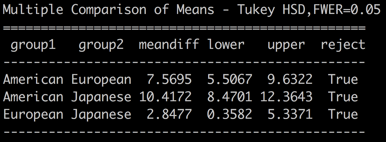
The table above shows the difference in mean for all the pairs of categories, the confidence intervals, and whether the null hypothesis is rejected or not.
Note how the MeanDiff correspond to the linear correlation coefficients that we obtained earlier.
The reject column is set to true for all the pairs, meaning that the difference in means is significant for all three pairs.
Summary
In this chapter, we tackled categorical variables as predictors. You saw that when the categories are not ordered naturally, it's necessary to transform the variable before adding it to the regression model. You learned how to:
Interpret the results of a univariate regression with categorical predictors.
Transform the predictor variable into dummy variables, a process also called one-hot encoding.
Apply binary encoding when facing large number of categories for a variable.
Run and interpret a one-way ANOVA test to determine the significance in the difference of means by group.
In the next chapter, you're going to learn how to apply linear regression to non-linear datasets by extending linear regression to polynomial regression. Fun and powerful stuff!
