Design Effective Statistical Models to Understand Your Data

12 hours
Medium

Free online content available in this course.

course.header.alt.is_video

course.header.alt.is_certifying

Last updated on 6/23/22

Build and Interpret a Polynomial Regression Model

Linear and logistic regression are powerful modeling techniques for regression and classification. However, they suffer from a major drawback; the assumption of linearity, which enforces a very strong approximation of the data. In the real world, linearity between variables is rare.

There are multiple ways to move beyond linearity using the context of linear regression. In this chapter, we will focus on polynomial regression, which extends the linear model by considering extra predictors defined as the powers of the original predictors.

At the end of this chapter, you will be able to:

Build polynomial regression models.
Select the best order of the polynomial.
Reduce structural multicollinearity
Understand the concept of overfitting.
Fit a quadratic interpolation with numpy.polyfit.

Polynomial Regression

Consider a univariate regression, where the outcome y is a function of a predictor X:

$$\[y = a X + b\]$$

You can extend that regression by adding powers of $$$X$$$ : $$$X^2$$$ , $$$X^3$$$ up to $$$X^p$$$ such that:

$$\[y = a_1 X + a_2 X^2 + \cdots + a_p X^p + b\]$$

You have created a polynomial of $$$X$$$ of order $$$p$$$ with $$$p \ge 2$$$ .

A polynomial regression is linear regression that involves multiple powers of an initial predictor.

Now, why would you do that? Two reasons:

The model above is still considered to be a linear regression. You can apply all the linear regression tools and diagnostics to polynomial regression.
Polynomial regression allows you to handle nonlinearities in the dataset. You are no longer constrained by the linearity assumption.

Let's look at a simple example.

The Dataset

We will work on a classic dataset used in statistic courses; the Ozone dataset, which consists of 111 observations of the following four variables:

Ozone: daily ozone concentration (ppb)
Radiation: solar radiation (Langley's)
Temperature: daily maximum temperature (degrees F)
Wind: wind speed (mph)

These observations were gathered over 111 days from May to September 1973 in New York. The target variable is the concentration of ozone.

As you will see, the relationships between ozone and wind and ozone and temperature is not entirely linear. So let's explore the data by plotting the relations between the variables with seaborn pairplot.

import pandas as pd
import seaborn as sns
df = pd.read_csv('ozone.csv')
# drop Day and Month columns and rename Solar.R as Solar
df= df.drop(columns = ['Day', 'Month']).rename(columns = {'Solar.R': 'Solar'})
sns.pairplot(df)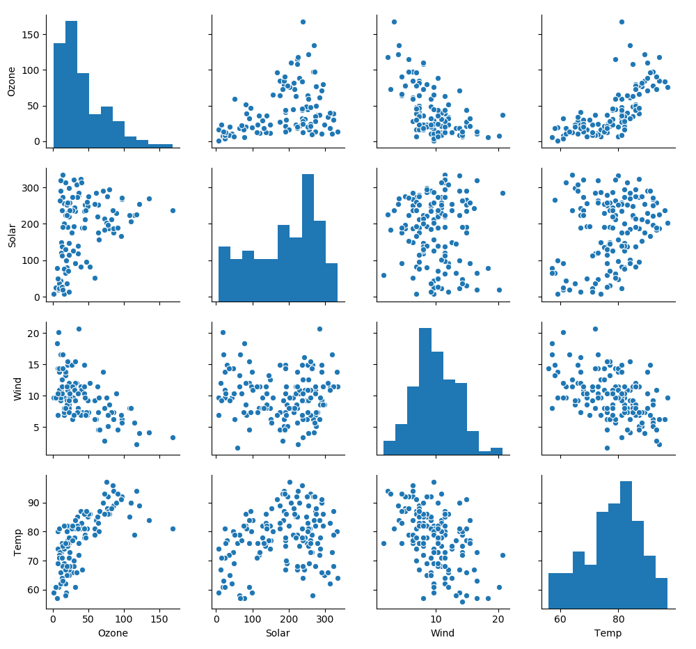

Scatter plots and histograms of the ozone dataset — Scatter plots and histograms of the Ozone dataset

These scatter plots are all far from being nice and linear. In particular, the curvature in the scatter plot Ozone vs. Wind is an indication of nonlinearity between the variables.

When do we need polynomial regression?

There's a reason to think that the relationship between the outcome and one of the predictors is not linear. You can assess this by looking at the scatter plot of the variables.

How Polynomial Should We Be?

The next question to answer is the maximum power of a variable we should add to the linear regression model. To illustrate the answer, we will compare three different models, each involving a different set of powers of the original variable.

Create a new variable as the square of the wind, and another as the cube of wind:

df['Wind2'] = df.Wind**2
df['Wind3'] = df.Wind**3

Build three models:

import statsmodels.formula.api as smf
M1 = smf.ols('Ozone ~ Wind ', df)
M2 = smf.ols('Ozone ~ Wind + Wind2', df)
M3 = smf.ols('Ozone ~ Wind + Wind2 + Wind3', df)

Let's compare the results with results.summary(). To save space, we're not reproducing the summary of the three models, but just focusing on the main metrics:

Model	Degree	R-squared	Log-likelihood	coefficients	p-values
M1	1	0.362	-543.6	$$$Wind$$$ : -5.5	9.2e-13
M2	2	0.486	-531.1	$$$Wind$$$ : -19.44, $$$Wind^2$$$ : 0.65	1.1e-10 8.3e-07
M3	3	0.498	-529.7	$$$Wind$$$ :-32.26 $$$Wind^2$$$ : 1.92 $$$Wind^3$$$ : -0.04	0.00017 0.016 0.105

These results show that adding new powers of the original variable does increase the performance of the model (R-squared increases, log-likelihood decreases). However, the p-values for the coefficients show that the coefficients M1 and M2 are reliable; but for M3, the p-value associated with $$$Wind^3$$$ is well above 0.05 and can't be trusted.

This case concludes that adding a square of the original variable improves the model, but adding another power no longer leads to a reliable model. The best degree for the polynomial is two.

Exercise: As an exercise, carry out the same analysis on the ozone vs. temp variable. Define three models:

M1: Ozone ~ Temp
M2: Ozone ~ Temp + Temp^2
M3: Ozone ~ Temp + Temp^2 + Temp^3

Compare the results of the three regressions. You should come to the conclusion that a second degree polynomial improves the model, but a third degree polynomial degrades it. The solution is in this lesson's screencast.

Selecting the Best Degree of the Polynomial

Selecting the best degree of the polynomial follows the same process as selecting the best model and set of predictors by analyzing the different metrics and statistics available in the regression summary.

Overfitting

Overfitting is an important concept in machine learning, which we will explore more in-depth in Part 4 of this course. Overfitting means that the model is so close and sensitive to the dataset, that it becomes ineffective for predicting new values, or for extrapolation.

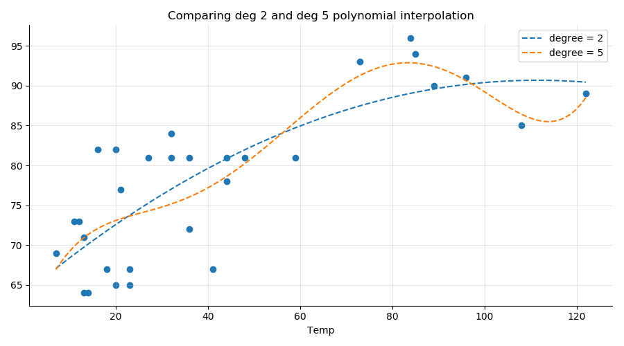
In the graph below, we compare a polynomial regression of degree 2 (blue line) with one of degree 5 (orange line) on a random subset (n = 30) of the Ozone ~ Wind data. As you can see, the degree 5 interpolation is very sensitive to the points on the right of the graph. If we were to use that degree 5 polynomial to make predictions based on new values, the accuracy would be worse than with the more robust 2nd-degree polynomial.

NumPy has a very convenient method called polyfit(), that can be used to find the coefficients of a polynomial of degree N to a couple of variables. For instance, to find the coefficients of a 2nd-degree polynomial fitting the Ozone ~ Temp relation, write:

# Ozone has some missing values
df = df.dropna().sample(n = 30)
q = np.polyfit(df.Ozone, df.Temp, 2)
print(q)
array([-1.39462928e-03,  4.48415581e-01,  6.33259214e+01])

Note also that the coefficients found by the np.polyfit method may not be the same ones as the regression coefficients for the equivalent model, as different methods are used in both libraries.

Selecting the optimum degree for a polynomial regression comes down to balancing the model’s complexity with its explanatory power. The best model is one that accomplishes the desired level of explanation or prediction with as few predictor variables as possible.

What About the Collinearity?

Consider our quadratic model: Ozone ~ Wind + Wind^2. The variables Wind and Wind^2 are very correlated:

r = np.corrcoeff(df.Wind, df.Wind2)
print("r = {:.2f}".format(r))
r = 0.97

It seems we have a violation of the collinearity assumption, which states that predictor variables should be decorrelated from one another for the linear regression to be reliable.

Fortunately, this is not the case.

What you see here is not multicollinearity related to the nature of the data where two predictors are correlated by chance as a consequence of some unknown confounder. We have a polynomial called structural correlation, and it is not a problem for linear regression.

Structural Correlation Is OK

We can show that structural correlation between predictors does not degrade the performance of the model.

One way to remove the correlation between $$$X$$$ and $$$X^2$$$ or between $$$X$$$ and some functions of $$$X$$$ is simply to center the variable $$$X_c = X - mean(X)$$$ . Then $$$X_c$$$ and $$$X_c^2$$$ are less correlated.

df['Wind_c'] = df.Wind - df.Wind.mean()
r = np.corrcoef(df.Wind_c, df.Wind_c**2 )
print("r = {:.2f}".format(r[0,1]))
r = 0.30

We see a very significant decrease in correlation.

If we build the model $$$M4: Ozone \sim Wind_c + Wind_c^2$$$ based on the centered variable $$$Wind_c$$$ , we get exactly the same results for M4 as we did for $$$M2: Ozone \sim Wind + Wind^2$$$ with the exception of the coefficients and associated statistics and confidence intervals. The correlation between the two predictors ( $$$Wind$$$ and $$$Wind^2$$$ ) has no impact on the overall quality of the linear model.

Summary

In this chapter, we used polynomial regression to bypass the constraint of linearity between the predictors and the outcome.

The key takeaways from this chapter are:

There's usually no reason to consider polynomials with degrees higher than three.
Correlation between the powers of a variable does not induce multicollinearity.
Selecting the best degree for the polynomial regression follows a similar model comparison process as with simple regression.
NumPy polyfit is a simple method for polynomial interpolation useful for graphic exploration.

This concludes Part 3 of the course! You should now be comfortable working with logistic regression, handling categorical variables, and tackling nonlinearities with polynomial regression.

In Part 4, we will work with linear and logistic regression to make predictions. We're moving away from statistical modeling and stepping into machine learning. Fun stuff, right?