Perform an Initial Data Analysis

Okay, so your friend gave you the average time of his trips, as well as the standard deviation. You can start to relax a little. But...here’s something you haven’t thought about.

Look at these two distributions:

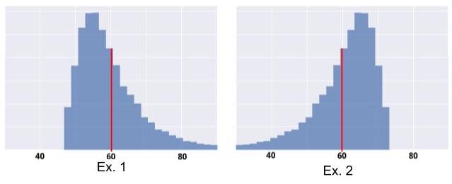
They have the same empirical mean (60 minutes), and the same standard deviation. However, Example 1 is “riskier” than Example 2. That’s right, in Example 2, it is highly unlikely that your trip will take more than 75 minutes: no risk of being late! But in Example 1, your trip could very well take 80 minutes, or even longer.

There are statistical measures for that! They are called Measures of Shape. 

Thinking It Through...

Let’s make our own shape indicator! We want to know if the distribution skews more to the left of the mean, or more to the right of it.

I suggest you take what we built in the last chapter. First, we had this idea:

Let’s take all of our values, and calculate the deviation from the mean for each one. Then let’s add these deviations together!

We expressed the deviation of a value from the mean as $\$\backslash ((x\_i\; -\; \backslash overline\{x\})\backslash )\$$. If this deviation is positive, it means that $\$\backslash (x\_i\backslash )\$$ is above the mean; if it is negative, it means that $\$\backslash (x\_i\; \backslash )\$$ is below the mean.

When we added all of these deviations together, we noticed that the result was always 0. So we squared the number: ( $\$\backslash ((x\_i\; -\; \backslash overline\{x\})^2\backslash )\$$ . With a squared number, the result is always positive. However, if it is always positive, we lose the information that tells us whether $\$\backslash (x\_i\backslash )\$$ is above or below the mean. And here, we want to keep that information!

Good idea! When we cube the deviation, we obtain $\$\backslash ((x\_i-\backslash overline\{x\})^3\backslash )\$$ . Unlike the squared number, the cubed number retains the negative sign of  $\$\backslash ((x\_i\; -\; \backslash overline\{x\})\backslash )\$$. Next, we take the average of all of these cubed deviations, and obtain: $\$\backslash (\backslash frac\{1\}\{n\}\backslash sum\_\{i=1\}^\{n\}(x\_i-\backslash overline\{x\})^3\backslash )\$$ .

We have achieved our goal: the amount will be negative if most of the values are below the mean; otherwise it will be positive!

But we can do even better. Take a look at these two distributions:

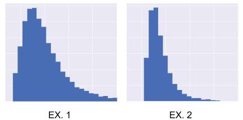
They have the same shape, but not the same standard deviation (distribution 1 is more spread out than distribution 2; distribution 1 has a standard deviation that is twice that of 2). Because they have the same shape, we would like for our indicator to have the same value for both distributions.

But currently, that’s not the case. In Example 1, the deviations from the mean are twice as great as in Example 2. Because we are cubing these deviations, our indicator will be $\$\backslash (2^3\backslash )\$$ greater for 1 than for 2. But we want them to be equal. So to correct this, we need to nullify the effect of the standard deviation. To do this, we are going to divide our indicator by the cubed standard deviation:

$\$\backslash [\backslash frac\{\backslash frac\{1\}\{n\}\backslash sum\_\{i=1\}^\{n\}(x\_i-\backslash overline\{x\})^3\}\{s^3\}\backslash ]\$$

Measures of Shape

Skewness

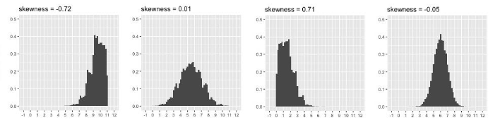
Guess what! The indicator we just created is commonly used by statisticians: it’s called Empirical Skewness. In general, skewness $\$\backslash (\backslash gamma\_1\backslash )\$$, and its numerator $\$\backslash (\backslash mu\_3\backslash )\$$ , are expressed:

$\$\backslash [\backslash gamma\_1\; =\; \backslash frac\{\backslash mu\_3\}\{s^3\}\backslash ]\$$

with $\$\backslash (\backslash mu\_3\backslash )\$$ =  $\$\backslash (\{\backslash frac\{1\}\{n\}\backslash sum\_\{i=1\}^\{n\}(x\_i-\backslash overline\{x\})^3\}\backslash )\$$ 

Skewness is a measure of asymmetry (or symmetry). The asymmetry of a distribution is the regularity (or lack thereof) with which the observations are distributed around a central value. It is interpreted as follows:

• • If $\$\backslash (\backslash gamma\_1=\; 0\backslash )\$$, the distribution is perfectly symmetrical.

• • If $\$\backslash (\backslash gamma\_1\; >\; 0\backslash )\$$, the distribution is positively skewed, or skewed right.

• • If , the distribution is negatively skewed, or skewed left.

Empirical Kurtosis

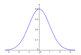
Empirical Kurtosis is not a measure of asymmetry; it’s a measure of “peakedness,” or “flatness.” Peakedness can be interpreted whenever the distribution is symmetrical. It is determined in relation to the most famous distribution of all: the so-called Normal Distribution (also known as the Gauss, Gaussian, or Bell Curve). I’m sure you’ve seen it. It looks like this:

Kurtosis is often expressed $\$\backslash (\backslash gamma\_2\backslash )\$$, and calculated by:

$\$\backslash [\backslash gamma\_2\; =\; \backslash frac\{\backslash mu\_4\}\{s^4\}-3\backslash ]\$$

with $\$\backslash (\backslash mu\_4\; =\; \backslash frac\{1\}\{n\}\backslash sum\_\{i=1\}^\{n\}(x\_i-\backslash overline\{x\})^4\backslash )\$$

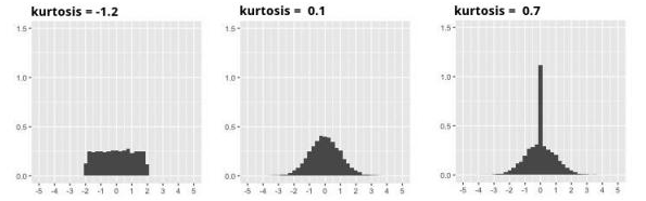
Kurtosis is interpreted as follows:

• If $\$\backslash (\backslash gamma\_2\; =\; 0\; \backslash )\$$, the distribution has the same degree of peakedness (or flatness) as the normal distribution.

• If $\$\backslash (\backslash gamma\_2\; >\; 0\backslash )\$$, the distribution is more peaked (less flat) than the normal distribution: the observations are more densely concentrated.

• If , the distribution less peaked (flatter) than the normal distribution: the observations are less densely concentrated.

Now for the code...

You know how it works! Take the code from the previous chapter and add some lines: here, 10 and 11, to calculate Skewness and Kurtosis:

for cat in data["categ"].unique():
    subset = data[data.categ == cat] # Creation of sub-sample
    print("-"*20)
    print(cat)
    print("mean:\n",subset['amount'].mean())
    print("med:\n",subset['amount'].median())
    print("mod:\n",subset['amount'].mode())
    print("var:\n",subset['amount'].var(ddof=0))
    print("ect:\n",subset['amount'].std(ddof=0))
    print("skw:\n",subset['amount'].skew())
    print("kur:\n",subset['amount'].kurtosis())
    subset["amount"].hist() # Creates the histogram
    plt.show()  # Displays the histogram
    subset.boxplot(column="amount", vert=False)
    plt.show()

Take It Further: A Word About Asymmetry

Remember this sentence from the beginning of the chapter?

“We want to see whether the majority of the values are above the mean or below the mean.”

When we say majority, we mean over 50% of the values. You will recall that the median is the middle value: 50% of the values are above it. Therefore, the above sentence is equivalent to saying: We want to know if the median is greater than or less than the mean.

A distribution is considered symmetrical if its shape is the same on either side of the center of the distribution. In this case: $\$\backslash (Mode\; =\; Med\; =\; \backslash overline\{x\}\backslash )\$$

A distribution is skewed right (or is positively skewed, or has positive asymmetry) if: .

Similarly, it is skewed left (or is negatively skewed) if: $\$\backslash (Mode\; >\; Med\; >\; \backslash overline\{x\}\backslash )\$$.

Take It Further: Moments

The Empirical Mean, Empirical Variance, $\$\backslash (\backslash mu\_3\backslash )\$$ and $\$\backslash (\backslash mu\_4\backslash )\$$ are all Moments.

The Mean, Variance, and Measures of Shape we have seen characterize the geometry of the distribution, which is what makes it similar to the definition of Moment of Inertia.

Indeed, people who study mechanics often calculate moments. For example, if you take a graduated ruler and attach a weight to each spot that corresponds to an observation $\$\backslash ((x\_1,...,x\_n)\backslash )\$$ , and then rotate this ruler about the mean value, the moment of inertia will be calculated the same way as the variance of $\$\backslash ((x\_1,...,x\_n)\backslash )\$$!

In statistics, the general empirical moment of order $\$\backslash (p\backslash )\$$ in relation to $\$\backslash (t\backslash )\$$ is given by the relation:

$\$\backslash [Mtp=1n\sum i=1n(xiat)p\backslash ]\$$

The simple empirical moment is the general moment about $\$\backslash (t=0\backslash )\$$

$\$\backslash [M\_p=\backslash frac\{1\}\{n\}\backslash sum\_\{i=1\}^\{n\}x\_i^p\backslash ]\$$

The central empirical moment is the general moment about the mean, or $\$\backslash (t=\backslash overline\{x\}\backslash )\$$: 

$\$\backslash [\backslash mu\_p=\backslash frac\{1\}\{n\}\backslash sum\_\{i=1\}^\{n\}(x\_i-\backslash overline\{x\})^p\backslash ]\$$