Train a Supervised Machine Learning Model

In machine learning, you use regression to predict continuous values such as temperature, stock price, and life expectancy.  Regression is a statistical technique that finds relationships between features.

Linear Regression

We will be looking at using sklearn's linear regression functionality in a subsequent chapter. You don't need to fully understand the math behind the algorithm to use it, but you should understand the concepts covered in this chapter as they are the foundation for a lot of machine learning techniques.

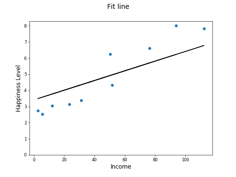
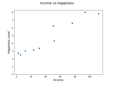
Let's consider a simplified version of the income versus happiness scatter plot and plot just 10 points:

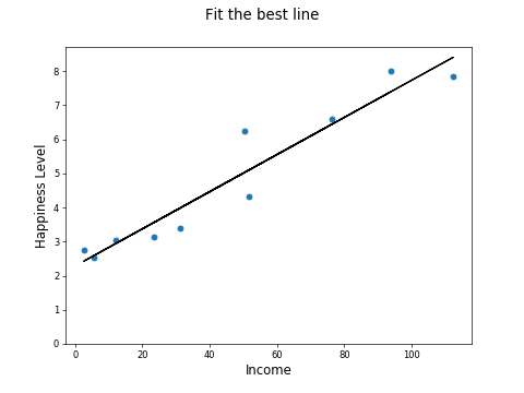
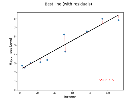
The big idea with linear regression is to fit a line to the data:

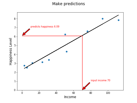
Make some predictions, such as here where we can predict that a country with an average income of $70k will have a happiness score of 5.51:

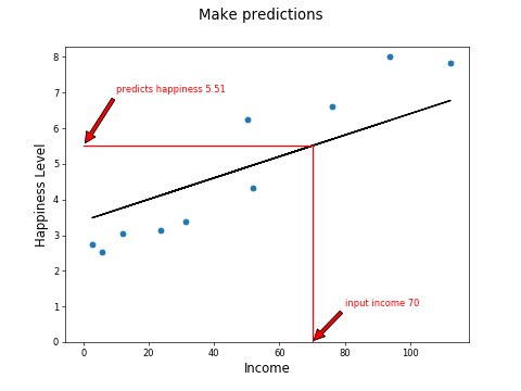
The line becomes a way to estimate the happiness from the income, effectively a machine learning model!

If you measure the distance from the points to the fitted line, you have a measure of how close the fitted line is to the actual, real-life data points:

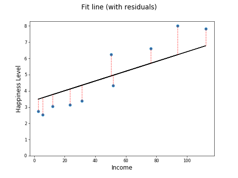
The distance between the fitted line and an actual point is called a residual.  The residuals for all the points are shown by the red dotted lines above.  Here are the residuals (i.e., the lengths of the red dotted lines):

-1.03
1.78
-0.72
0.9
-0.74
1.06
-0.65
-0.95
-0.99
1.33

The length of any one residual line tells you how good the model is estimating the happiness value for that sample point. So naturally, the total length of all the residual lines tells you how good the model is at estimating the happiness value from all the sample points. But, if you add up all the numbers above, the negative and positive values will tend to cancel each other out. 

-1.03 + 1.78 + -0.72 + 0.9 + -0.74 + 1.06 + -0.65 + -0.95 + -0.99 + 1.33 =
Total: 0.01

So, a better way would be to take the absolute values and sum those:

1.03
1.78 
0.72
0.9
0.74
1.06
0.65
0.95
0.99
1.33
Total: 10.15

In this way, you are just looking at the magnitude of the residual and ignoring whether it is above or below the line. After all, an error of 1.03 is as significant, whether it's an overestimate or an underestimate.

Another way to eliminate the sign is to square each value and sum the squares.  Let's square the original signed residuals and sum them:

1.0609
3.1684
0.5184
0.81
0.5476
1.1236
0.4225
0.9025
0.9801
1.7689
Total: 11.30

In general, use the squaring method rather than the absolute value method. This is the measure of how good a fit your line is. It's called the sum of squared residuals, or SSR. It's also sometimes called the sum of squared errors, or SSE.

So, now you have a way of measuring the first attempt at fitting a line, let's try out a few others:

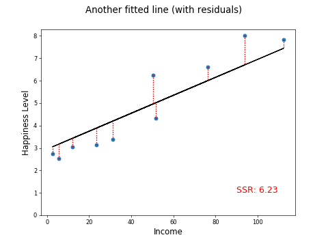
Much better!

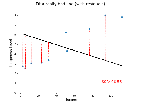
Much worse!!

Now, you are probably thinking that there must be a better way to find the best fitting line than trying them out one-by-one.  You're right!  It's called the ordinary least squares method (OLS method).

Ordinary Least Squares

You may remember from your school math lessons the formula for a straight line:

y = mx + c

where m is the slope of the line, and c is the intercept on the y axis.

If m= 0.5 and c = 20, you get the following function:

y = 0.5x + 20

Let's plot that function:

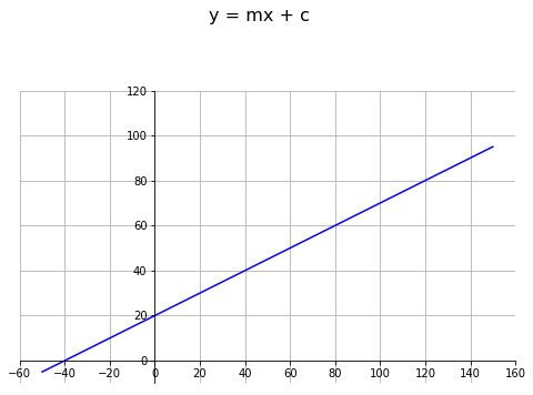
The line crosses the y-axis at y=20. This is the intercept c in our formula and the slope is 1 in 2. This is the slope, m is the formula for a line.

To define any line, we need to specify the right values for m and c. Looking back to our set of points:

Find the values of m and c, which minimizes the sum of squared residuals to these points. Easier said than done! Fortunately, some formulae do just that. Here's how to compute the slope:

$\$\backslash [m\; =\; \backslash frac\{\backslash Sigma\; ((x-\backslash bar\{x\})\; \backslash times\; (y\; -\backslash bar\{y\}))\}\{\backslash Sigma(x-\backslash bar\{x\})^2\}\; \backslash ]\$$

And here's how to compute the y intercept:

$\$\backslash [c\; =\; \backslash bar\{y\}\; -\; m\; \backslash times\; \backslash bar\{x\}\backslash ]\$$

Here is a simple Python function that implements these formulae, given a set of points in the arrays x and y:

def ols(x, y):
    xmean = x.mean()
    ymean = y.mean()
    xvariance = sum([(x - xmean)**2 for x in x])
    xycovariance = 0
    for i in range(len(x)):
        xycovariance += (x[i] - xmean) * (y[i] - ymean)
    m = xycovariance / xvariance
    c = ymean - m * xmean
    return m, c

Plugging the five sample points into this function, you get:

m = 0.05442586953454801
c = 2.283356593384597

And plugging m and c into the general formula for a straight line, you get:

y= 0.05442586953454801 * x + 2.283356593384597

Let's plot the line:

This is the line of best fit using the OLS method.

Just to prove this is better than the other lines, let's plot the residuals and calculate the SSR:

This beats our previous best SSR of 6.23.

Making Predictions

The whole point of this exercise is to build a model to make predictions.  Now that we have a formula for the line, we have a formula for predicting happiness from income!

 happiness = 0.05442586953454801 * income + 2.283356593384597

To predict happiness from an income of 70:

happiness = 0.05442586953454801 * 70 + 2.283356593384597 = 6.09

And here is the graphical representation of the above:

Multiple Regression

So far, in this chapter, we have only discussed situations where we are predicting a value from another single feature. To do this, we fitted a line using the formula:

y = mx + c

But what if there are two or more input features?

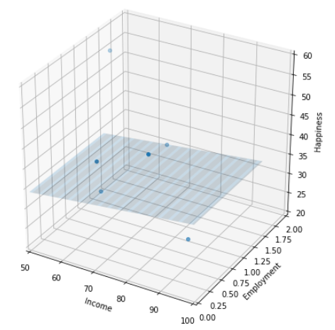
For two input features, the formula looks like this:

$\$\backslash (y\; =\; m\_1x\_1\; +\; m\_2x\_2\; +\; c\backslash )\$$

Instead of describing a line, it describes a two-dimensional plane.  We need this formula to predict happiness from both income and employment levels.

The regression task changes from "fitting a line that best predicts happiness from income," to "fitting a 2D plane that best predicts happiness from income and employment levels:"

For three input features, the formula looks like this:

$\$\backslash (y\; =\; m\_1x\_1\; +\; m\_2x\_2\; +\; m\_3x\_3\; +\; c\backslash )\$$

We are fitting a 3D plane to the data!

In other words, for each new feature you add, you need to compute an additional slope m, and we increase the dimensionality of the fitted plane.

Recap

• Linear regression works by fitting a line to a set of data points.

• You can measure the distance from the line to your actual data points. These are called residuals.

• Find your total error by summing the squares of the residuals for all data points.  This is called the sum of squared residuals, or SSR.

• The ordinary least squares (OLS) method finds the optimal fitting line by minimizing the SSR.

• Use the line computed using the OLS method to predict one feature (the y-axis) from the other feature (the x-axis).

• Extend the approach to use multiple input features. This is called multiple regression.

 In the next chapter, we will take a look at the KNN algorithm.