Train a Supervised Machine Learning Model

Now that you have an understanding of a couple of regression algorithms (namely, linear regression and k-nearest neighbors), let's build some regression models in Python.

We will follow the same process used previously for our classification tasks:

We will use the same world indicators dataset, so refer back to Part 3, Chapter 3, for a reminder of the origins and description of this data.

Import the Necessary Libraries

Let's start by importing the necessary libraries - pandas, NumPy, and matplotlib, as well as some sklearn functions. We will also import a small library of convenience functions used specifically for this course. Feel free to open up functions.py to see what's inside.

# Core libraries
import pandas as pd
import numpy as np
import matplotlib.pyplot as plt

# Sklearn processing
from sklearn.preprocessing import MinMaxScaler
from sklearn.model_selection import train_test_split

# Sklearn regression algorithms
from sklearn.linear_model import LinearRegression
from sklearn.neighbors import KNeighborsRegressor
from sklearn.tree import DecisionTreeRegressor

# Sklearn regression model evaluation function
from sklearn.metrics import mean_absolute_error

# Convenience functions.  This can be found on the course github
from functions import *

Define the Task

The task is:

Make predictions about a country's life expectancy in years from a set of metrics for the country.

The only difference between this task and the one we defined for our classification task is that we are predicting the life expectancy in years, rather than as L, M, and H bands. Remember that regression is about predicting a continuous numeric feature and classification is about predicting a category.

Acquire Clean Data

This is the same data used for the classification task, so I'm going to quickly clean it up using the same code used in that task:

# Load the data
dataset = pd.read_csv("world_data.csv")

# Remove sparsely populated features
dataset = dataset.drop(["murder","urbanpopulation","unemployment"], axis=1)

# Impute all features with mean
means = dataset.mean().to_dict()
for m in means:
    dataset[m] = dataset[m].fillna(value=means[m])

Understand the Data

We spent some time in Part 3, Chapter 3, inspecting and visualizing this data.  I won't repeat that here, but I will introduce some other interesting visualizations.

First, a little bonus!  If you run the following, you will get a list of alternative styles for your charts:

print(plt.style.available)

['bmh', 'classic', 'dark_background', 'fast', 'fivethirtyeight', 'ggplot', 'grayscale', 'seaborn-bright', 'seaborn-colorblind', 'seaborn-dark-palette', 'seaborn-dark', 'seaborn-darkgrid', 'seaborn-deep', 'seaborn-muted', 'seaborn-notebook', 'seaborn-paper', 'seaborn-pastel', 'seaborn-poster', 'seaborn-talk', 'seaborn-ticks', 'seaborn-white', 'seaborn-whitegrid', 'seaborn', 'Solarize_Light2', 'tableau-colorblind10', '_classic_test']

You can then select one of the styles to make your charts look a little nicer!

plt.style.use('bmh')

You can understand the distribution of each individual feature using histograms:

dataset.hist(figsize=(20,20))
plt.show()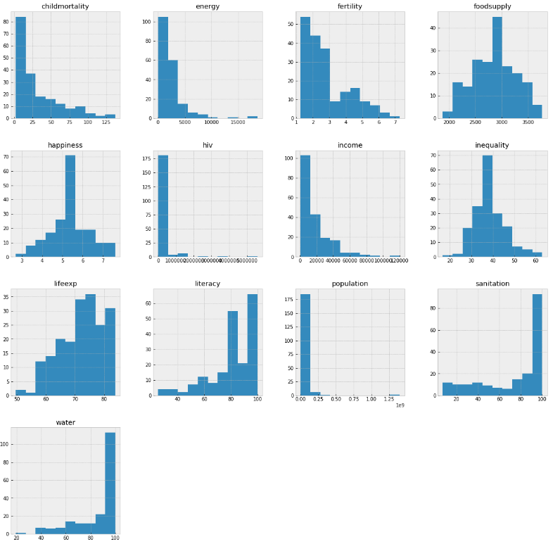 

Another interesting plot is the scatter matrix.  This shows the correlation between pairs of features:

scatterMatrix(dataset)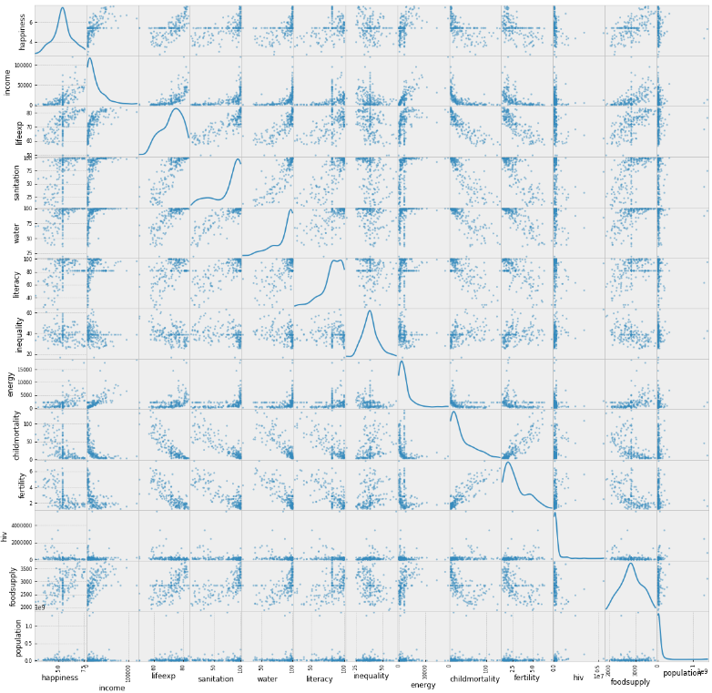

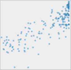
For example, you can look at the correlation between lifeexp and sanitation and see a positive correlation:

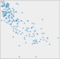
And lifeexp and fertility and see a negative correlation:

Again, this gives you a better feel for the data, and in particular, how the target feature, lifeexp, relates to the other features. After all, this is the relationship the machine learning algorithms will use to make their predictions!

Prepare Data

Select Features and Split Into Input and Target Features

We will predict lifeexp, and this feature becomes our y.  We will use all the other features as our inputs, X:

y = dataset["lifeexp"]
X = dataset[['happiness', 'income', 'sanitation', 'water', 'literacy', 'inequality', 'energy', 'childmortality', 'fertility',  'hiv', 'foodsupply', 'population']]

Scale Features

As discussed in the classification exercise performed with this data, scale the data before building the model to ensure the features are presented without a scale bias to the selected algorithms.

In this case, I will use the MinMaxScaler(), which scales the data, so every feature sits in the range 0 to 1.

# Rescale the data
scaler = MinMaxScaler(feature_range=(0,1))
rescaledX = scaler.fit_transform(X)

# Convert X back to a Pandas DataFrame, for convenience
X = pd.DataFrame(rescaledX, index=X.index, columns=X.columns)

Build Models

You learned about two algorithms for regression: linear regression and k-nearest neighbors. We will build models using both of these. I will also build a model with another algorithm, support vector machine.  We haven't explored this yet, but sklearn makes it easy to try new algorithms. We can try it out and explore further if it looks promising!

Split Into Test and Training Sets

We will build all three models using the same training set and evaluate them with the same test set.  So, let's split into test and training sets now:

test_size = 0.33
seed = 1
X_train, X_test, Y_train, Y_test = train_test_split(X, y, test_size=test_size, random_state=seed)

Create Multiple Models, Fit and Check Them

Let's build the models. I'll take a slightly different approach this time, to reduce the amount of coding when building and evaluating multiple models. First, I'll create a list of the untrained models. SVR is the support vector machine model (SVR stands for support vector regressor).

models = [LinearRegression(), KNeighborsRegressor(), SVR()]

Now, I will loop through all the models and fit them to the data:

for model in models:
    model.fit(X_train, Y_train)
    predictions = model.predict(X_train)
    print(type(model).__name__, mean_absolute_error(Y_train, predictions))

LinearRegression 2.2920035925091753

KNeighborsRegressor 2.1955055341375442 

SVR 3.6117510998705655

You can see the mean absolute error (MAE) for each model based on the training data. The MAE is the mean of the sum of the absolute values of all prediction errors. In other words, for each prediction, subtract the predicted value from the actual value, take the absolute value, sum up all these, and divide by the number of examined sample points:

$\$\backslash (MAE\; =\; \backslash frac\; \{\backslash Sigma\; \backslash vert\; y\; -\; \backslash hat\{y\}\; \backslash vert\}\{N\}\backslash )\$$

Where y is the actual value, ŷ is the predicted value, and N is the number of sample points.

In this case, the values are in the units of the predicted feature, which is life expectancy in years. So linear regression has achieved a mean absolute error of 2.29 years. As this is on the training data, we now need to use the test data to do a proper evaluation. 

Evaluate Models

Now we evaluate the models by testing with the test set:

for model in models:
    predictions = model.predict(X_test)
    print(type(model).__name__, mean_absolute_error(Y_test, predictions))

 LinearRegression 2.4463956508110285

KNeighborsRegressor 2.5532340600575907

SVR 3.6854103854533866

Which is the best model?  The one with the lowest mean absolute error, which is linear regression.  So we will choose this model:

model = models[0]

To get a better feel for how well the model has worked, we can add the predictions and actuals back to the test data, so we can see the quality of the predictions on a country-by-country basis:

predictions = model.predict(X_test)
df = X_test.copy()
df['Prediction'] = predictions
df['Actual'] = Y_test
df["Error"] = Y_test - predictions
df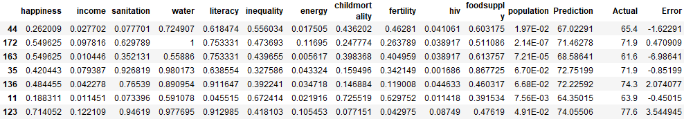

Look at the three columns on the far right of the above table.  These show how close the model is to predicting the actual life expectancy for each country.

Iterate!

At this point, you will want to go back to previous steps such as cleansing and feature engineering, to attempt to make improvements to the model.

Inspect the Models

It's good to look inside the models to understand what was created. Linear regression and KNN use very different ways of building models, and you need to interpret them in different ways.

Linear Regression

Interpreting a linear regression model is easy!  Use the  linearRegressionSummary()  function in  functions.py  to generate a chart of the coefficients:

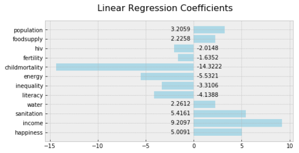
How do you interpret this?

For each unit increase in happiness, there is a 5.0091-year increase in lifeexp. 

For each unit increase in income, there is a 9.2097- year increase in lifeexp.

For each unit increase in inequality, there is a 3.3106-year decrease in lifeexp.

Be aware of what a "unit" means in this case. Because we scaled the data using the MinMaxScaler, all features are the scaled units. So one unit of income is the difference between the max income ($120,000), and min income ($623), which is $119,377. If you do the math (119377/9.2097), you can see that this model predicts that each $12,962 increase in average income, increases life expectancy by one year.

Extract the coefficients using this code:

models[0].coef_

array([ 5.00912637, 9.2096769 , 5.41605897, 2.26122297, -4.13876626, -3.31059309, -5.53211396, -14.32217202, -1.63521978, -2.01476135, 2.22581396, 3.20586791])

Extract the intercept using this code:

models[0].intercept_

69.60409836404611

Relate these directly back to the formula for a line we used in our exploration of linear regression:

$\$\backslash (y\; =\; m\_1x\_1\; +\; m\_2x\_2\; +\; m\_3x\_3\; +\; ...+\; c\backslash )\$$

In our case, y is lifeexp, m1 is the first coefficient (for happiness); m2 is the second coefficient (for income), etc.; x1, x2, etc., are the input features (happiness, income, etc.) themselves. Finally, c is the intercept.

The  formula for the linear regression line computed by sklearn from this data is:

lifeexp =
        5.00912637*happiness
     + 9.2096769*income
     + 5.41605897*sanitation
     + 2.26122297*water
     + -4.13876626*literacy
     + -3.31059309*inequality
     + -5.53211396*energy
     + -14.32217202*childmortality
     + -1.63521978*fertility
     + -2.01476135*hiv
     + 2.22581396*foodsupply
     + 3.20586791*population
     + 69.60409836404611 

Remember that the inputs to this formula are the scaled inputs, using the MinMaxScaler.

K-Nearest Neighbors

Interpreting KNN models is a little more tricky. The problem isn't reduced to a simple formula. The algorithm performs a calculation for each individual.

We can get the distances for the k-nearest neighbors for each data point:

models[1].kneighbors(X)

 (array([[0. , 0.38911668, 0.3929857 , 0.4201251 , 0.51618381],
[0. , 0.20505552, 0.20891422, 0.23226123, 0.26827204],
[0. , 0.12274953, 0.1953064 , 0.22064946, 0.22207317],
[0. , 0.16349608, 0.20891422, 0.22826679, 0.28847733],
[0.13327753, 0.15176936, 0.16216559, 0.16956607, 0.18772587],
[0.10256832, 0.15520456, 0.24629633, 0.24943538, 0.25508778],
[0. , 0.3593436 , 0.38793799, 0.38953126, 0.39317685],
...

As you can see, there are five values for each data point because that is the default value of k for the KNeighborsRegressor.

We can also get the actual data points that are the nearest neighbors:

g = models[1].kneighbors_graph(X).toarray()

Inspecting the neighbors of the first data point:

g[0]

array([0., 0., 0., 0., 0., 0., 0., 0., 0., 0., 1., 0., 0., 0., 0., 0., 0., 0., 0., 0., 0., 0., 0., 0., 0., 0., 0., 0., 0., 0., 0., 0., 0., 0., 0., 0., 1., 0., 0., 0., 0., 0., 0., 0., 0., 0., 1., 0., 0., 0., 0., 0., 0., 0., 0., 0., 0., 0., 1., 0., 0., 0., 0., 0., 0., 0., 0., 0., 0., 0., 0., 0., 0., 0., 0., 0., 0., 0., 0., 0., 0., 0., 0., 0., 0., 0., 0., 0., 0., 0., 0., 0., 0., 0., 0., 0., 0., 0., 0., 0., 0., 0., 0., 0., 0., 0., 0., 0., 1., 0., 0., 0., 0., 0., 0., 0., 0., 0., 0., 0., 0., 0., 0., 0., 0., 0., 0., 0., 0.])

Each 1 represents another data point that is considered a neighbor.  As you can see, there are five because that is the default value of k for the KNeighborsRegressor.

Recap

• Build multiple models from the same dataset, and see which one performs the best.

• Measure the performance of a regression model using mean absolute error (MAE).

• Iterate to improve model performance.

• Inspect the coefficients for a linear regression model, and use them to understand the relevance of each input feature to the predictions of the model.

• Inspect the information about the neighbors in a KNN model, but these are more difficult to interpret.

You've made it! What an excellent achievement. Before I wish you a final farewell (and hopefully, see you very soon ;)), I encourage you to take the very last quiz that will test your knowledge about building a regression model.  You're well on your way to become a Machine Learning expert! Keep it up.