Improve the Performance of a Machine Learning Model

In this chapter, we will examine some metrics for evaluating regression algorithms. I will be throwing in some math to help the explanation, but I will also explain things using examples that should be clear even if the math isn't.

Use Mean Absolute Error (MAE)

In the previous course, Train a Supervised Machine Learning Model, we evaluated the performance of regression models by computing the mean absolute error (MAE). We defined the MAE as

$\$\backslash [MAE\; =\; \backslash frac\; \{\backslash Sigma\; \backslash vert\; y\; -\; \backslash hat\{y\}\; \backslash vert\}\{N\}\backslash ]\$$

where $\$\backslash (y\backslash )\$$ is the actual value $\$\backslash (ŷ\backslash )\$$ is the predicted value and $\$\backslash (\backslash vert\; y\; -\; \backslash hat\{y\}\; \backslash vert\backslash )\$$ is the absolute value of the difference between the actual and predicted value. N is the number of sample points.

Let's dig into this a bit deeper to understand what this calculation represents.

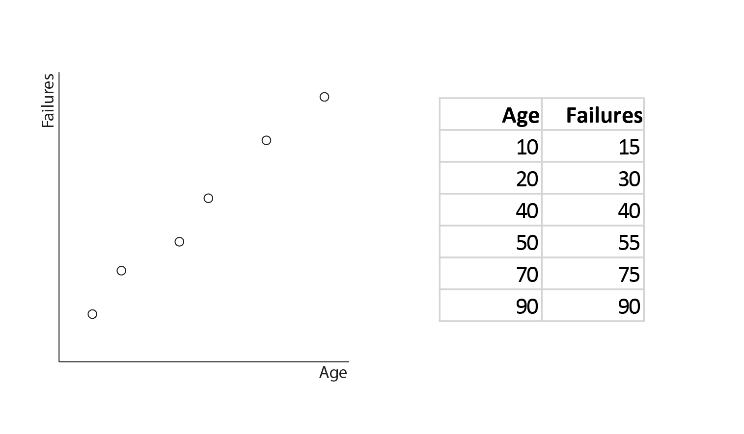
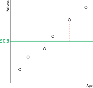
Take a look at the following plot, which shows the number of failures for a piece of machinery against the age of the machine:

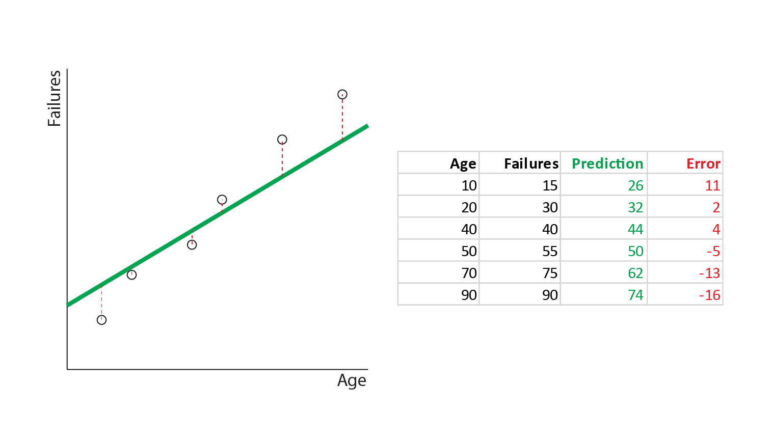
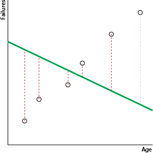
In order to predict the number of failures from the age, we would want to fit a regression line such as this:

In order to understand how well this line represents the actual data, we need to measure how good a fit it is. We can do this by measuring the distance from the actual data points to the line:

 You may recall that these distances are called residuals or errors. The mean size of these errors is the MAE. We can calculate it as follows:

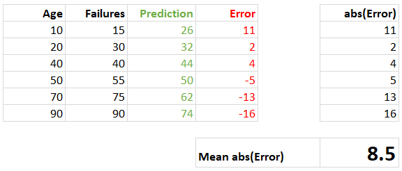
The mean of the absolute errors (MAE) is 8.5.

If mathematical symbols are not your strong point, you may not immediately see how this calculation relates to the formula at the start of this chapter:

$\$\backslash [MAE\; =\; \backslash frac\; \{\backslash Sigma\; \backslash vert\; y\; -\; \backslash hat\{y\}\; \backslash vert\}\{N\}\backslash ]\$$

So here is how the table and formula relate:

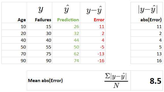
The MAE has a big advantage in that the units of the MAE are the same as the units of $\$\backslash (y\backslash )\$$, the feature we want to predict. In the example above, we have an MAE of 8.5, so it means that on average our predictions of the number of machine failures are incorrect by 8.5 machine failures. This makes MAE very intuitive and the results are easily conveyed to a non-machine learning expert!

Use Root Mean Square Error (RMSE)

Another evaluation metric for regression is the root mean square error (RMSE). Its calculation is very similar to MAE, but instead of taking the absolute value to get rid of the sign on the individual errors, we square the error (because the square of a negative number is positive).

The formula for RMSE is:

$\$\backslash [RMSE\; =\; \backslash sqrt\; \backslash frac\; \{\backslash Sigma\; (\; y\; -\; \backslash hat\{y\}\; )^2\}\{N\}\backslash ]\$$

Here is the calculation for RMSE on our example scenario:

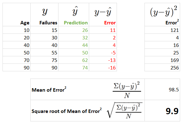
As with MAE, we can think of RMSE as being measured in the y units. So the above error can be read as an error of 9.9 machine failures on average per observation.

MAE vs. RMSE

Compared to MAE, RMSE gives a higher total error and the gap increases as the errors become larger. It penalizes a few large errors more than a lot of small errors. If you want your model to avoid large errors, use RMSE over MAE.

You should also be aware that as the sample size increases, the accumulation of slightly higher RMSEs than MAEs means that the gap between these two measures also increases as the sample size increases.

Use R-Squared

I stated above that an advantage of both MAE and RMSE is that they can be thought of as errors in the units of $\$\backslash (y\backslash )\$$, the predicted feature. This is helpful when relaying the results to non-data scientists. We can say things like "our model can predict the reliability of our machinery to within 8.5 machine failures on average" or "our model can predict the selling price of a house to within £15k on average".

It says nothing about whether an error of 8.5 machine failures or an error of £15k on a house price is good or bad. We can't compare how good different models are for different scenarios.

This is where R-squared or $\$\backslash (R^2\backslash )\$$ comes in. Here is the formula for $\$\backslash (R^2\backslash )\$$ :

$\$\backslash [R^2\; =\; \backslash frac\; \{\backslash Sigma\; \{(y\; -\; \backslash bar\; y)^2\}\; -\; \backslash Sigma\; \{(y\; -\; \backslash hat\; y)^2\}\}\{\backslash Sigma\; \{(y\; -\; \backslash bar\; y)^2\}\}\backslash ]\$$

$\$\backslash (R^2\backslash )\$$ computes how much better the regression line fits the data than the mean line. Another way to look at this formula is to compare the variance around the mean line to the variation around the regression line:

$\$\backslash [R^2\; =\; \backslash frac\; \{var(mean)\; -\; var(line)\}\{var(mean)\}\backslash ]\$$

Take our example above, predicting the number of machine failures. We can examine the errors for our regression line as we did before. We can also compute a mean line (by taking the mean $\$\backslash (y\backslash )\$$ value) and examine the errors against this mean line. That is to say, we can see the errors we would get if our model just predicted the mean number of failures (50.8) for every age input. Here are the regression and mean lines, and their respective errors:

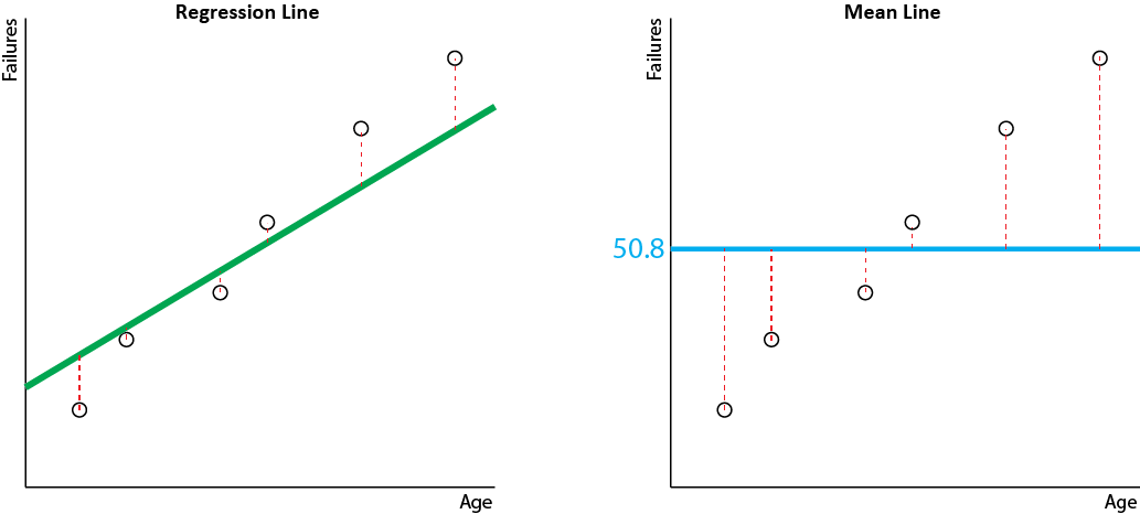
You can see that the regression line fits the data better than the mean line, which is what we expected (the mean line is a pretty simplistic model, after all). But can you say how much better it is? That's exactly what $\$\backslash (R^2\backslash )\$$ does! Here is the calculation.

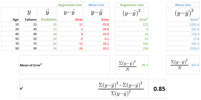
The additional parts to the calculation are the column on the far right (in blue) and the final calculation row, computin  $\$\backslash (R^2\backslash )\$$.

So we have an R-squared of 0.85. Without even worrying about the units of $\$\backslash (\; y\backslash )\$$ we can say this is a decent model. Why? Because the model explains 85% of the variation in the data. That's exactly what an R-squared of 0.85 tells us!

Here's another example. What if our data points and regression line looked like this?

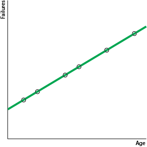
The variance around the regression line is 0. In other words, var(line) is 0. There are no errors.

Now, remember that the formula for R-squared is:

$\$\backslash [R^2\; =\; \backslash frac\; \{var(mean)\; -\; var(line)\}\{var(mean)\}\backslash ]\$$

So, with var(line) = 0 the above calculation for R-squared is

$\$\backslash [R^2\; =\; \backslash frac\; \{var(mean)\; -\; 0\}\{var(mean)\}\; =\; \backslash frac\; \{var(mean)\}\{var(mean)\}\; =\; 1\backslash ]\$$

Let's look at another example. What if our data points and regression line looked like this, with the regression line equal to the mean line?

In this case, var(line) and var(mean) are the same. So the above calculation will yield an R-squared of 0:

$\$\backslash [R^2\; =\; \backslash frac\; \{var(mean)\; -\; var(mean)\}\{var(mean)\}\; =\; \backslash frac\; \{0\}\{var(mean)\}\; =\; 0\backslash ]\$$

What if our regression line was really bad, worse than the mean line?

It's unlikely to get this bad! But if it does, var(mean)-var(line) will be negative, so R-squared will be negative.

I hope you can see that R-squared is a really useful evaluation metric for regression models.

Calculate These Evaluation Metrics With Python

Sklearn makes using these evaluation metrics with your models very straightforward. Here are the three functions you need. For each function just pass in the actuals and predictions

# MAE
mean_absolute_error(actuals, predictions)

# RMSE
sqrt(mean_squared_error(actuals, predictions)

# R-Squared
r2_score(actuals, predictions)

A complete example of a model build and evaluation is shown below. It uses a slightly modified version of UCI's "Boston" dataset, which can be used to experiment with building regression models that predict house prices.

The Jupyter notebook containing this example code can be found on the course Github repository.

If you need to, refer back to the previous course Train a Supervised Model, for a reminder of the steps in training a supervised model.

First, let's import the functions we need:

# Core libraries
import pandas as pd

# Sklearn processing
from sklearn.preprocessing import MinMaxScaler
from sklearn.model_selection import train_test_split

# Sklearn regression algorithms
from sklearn.linear_model import LinearRegression
from sklearn.neighbors import KNeighborsRegressor

# Sklearn regression model evaluation functions
from sklearn.metrics import mean_absolute_error
from sklearn.metrics import mean_squared_error
from math import sqrt
from sklearn.metrics import r2_score

Now load the data set:

# Load Boston housing data set
boston = pd.read_csv("boston.csv")

Let's take a look at the data by converting the built-in data set to a Pandas dataframe:

# View the features
boston.head()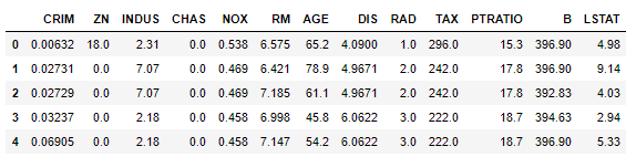

Select the features to use in our model:

# Define the X (input) and y (target) features
X = boston.drop("MEDV", axis=1)
y = boston["MEDV"]

Scale the input features, to avoid problems with variation in the scale of different features.

# Rescale the input features
scaler = MinMaxScaler(feature_range=(0,1))
X = scaler.fit_transform(X)

Split the data into training and test sets:

# Split into train (2/3) and test (1/3) sets
test_size = 0.33
seed = 7
X_train, X_test, y_train, y_test = train_test_split(X, y, test_size=test_size, random_state=seed)

Build and check the models using the training data:

# Build some models and check them against training data using MAE, RMSE and R2
models = [LinearRegression(), KNeighborsRegressor()]
for model in models:
    model.fit(X_train, y_train)
    predictions = model.predict(X_train)
    print(type(model).__name__)
    print("    MAE", mean_absolute_error(y_train, predictions))
    print("    RMSE", sqrt(mean_squared_error(y_train, predictions)))
    print("    R2", r2_score(y_train, predictions))

LinearRegression
    MAE 3.320553824991157
    RMSE 4.669735688876091
    R2 0.7538411248592967
KNeighborsRegressor
    MAE 2.5493215339233037
    RMSE 3.921007185039673
    R2 0.8264493776882362

Evaluate the models using the test data:

# Evaluation the models against test data using MAE, RMSE and R2
for model in models:
    predictions = model.predict(X_test)
    print(type(model).__name__)
    print("    MAE", mean_absolute_error(y_test, predictions))
    print("    RMSE", sqrt(mean_squared_error(y_test, predictions)))
    print("    R2", r2_score(y_test, predictions))

 LinearRegression
    MAE 3.4097336094727595
    RMSE 5.086878583324625
    R2 0.6590081405512094
KNeighborsRegressor
    MAE 3.0038323353293412
    RMSE 4.546077074408997
    R2 0.7276578531589541

Summary

• Mean Absolute Error (MAE) tells us the average error in units of $\$\backslash (y\backslash )\$$ , the predicted feature. A value of 0 indicates a perfect fit. 

• Root Mean Square Error (RMSE) indicates the average error in units of $\$\backslash (y\backslash )\$$ , the predicted feature, but penalizes larger errors more severely than MAE. A value of 0 indicates a perfect fit. 

• R-squared ($\$\backslash (R^2\backslash )\$$ ) tells us the degree to which the model explains the variance in the data. In other words how much better it is than just predicting the mean. 

  • A value of 1 indicates a perfect fit.

  • A value of 0 indicates a model no better than the mean. 

  • A value less than 0 indicates a model worse than just predicting the mean.

• Python does the hard work and calculates these metrics for us from our model outputs.

And that's it for part 2! Ready to put your newfound knowledge to the test? Then let's go!