Improve the Performance of a Machine Learning Model

When it comes to adding input features to our model, quality is far more important than quantity. In this chapter, we will look at ways to select quality features from our dataset.

Become Selective

When faced with a number of possible input features, we want to ensure we choose really good features to train our model. This can become increasingly difficult when we have a data set with a high number of input features (datasets which we call high-dimensionality).

So far we have been using our own judgment when selecting the features to use in our models. But making bad decisions when making these selections can lead to underperforming models! Eek.

It is tempting to just throw all the available features at the algorithm and leave it to decide what to do. However, this can cause a few problems such as:

• Overfitting of the model

• Increased training time, as the more input features we have the harder the algorithm needs to work to make sense of them

• Inaccuracy, due to the presence of misleading data

• Difficulty interpreting the model, due to the complexity and high number of input features

Fortunately, there are ways to make a more informed choice of which features to select for our model which addresses these problems.

There are three general approaches to feature selection:

• Filter methods

• Wrapper methods 

• Embedded methods

We often use a filter method to quickly eliminate particularly poor features, and then use a wrapper or embedded method.

In this chapter, we will carry out some feature selection using the Boston house prices dataset. Here is the code that loads this data, splits into $\$\backslash (X\backslash )\$$ and $\$\backslash (y\backslash )\$$ , and scales the $\$\backslash (X\backslash )\$$ .

# Core libraries
import pandas as pd

# Sklearn processing
from sklearn.preprocessing import MinMaxScaler
from sklearn.model_selection import train_test_split

# Load Boston housing data set
boston = pd.read_csv("boston.csv")

# Define the X (input) and y (target) features
X = boston.drop("MEDV", axis=1)
y = boston["MEDV"]

# Rescale the input features
scaler = MinMaxScaler(feature_range=(0,1))
X_ = scaler.fit_transform(X)
X = pd.DataFrame(X_, columns=X.columns)

Here is a reminder of the structure of the input features:

# View the input features
X.head()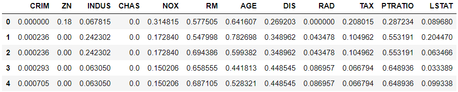

The following sections give different treatment to this data in order to illustrate different feature selection techniques.

Use Filter methods

Filter methods can be used as part of the data preparation process. The method used is independent of the machine learning algorithm we will be using.

Filter methods process the data very quickly. They work by ranking features based on some criteria and removing features that fall below a certain threshold.

Univariate methods rank features independently of other features. 

Multivariate methods select features by looking at features in relation to each other. For example, we can look at the correlation between features. This can address issues like multicolinearity. 

Remove Low Variance Features

Sklearn provides the VarianceThreshold() function to remove less important features. It uses variance as the ranking criteria. We can use it to remove features that are constant (have a variance of 0, i.e. all rows have the same value) or nearly constant (have a variance that is very low).

First, we split our $\$\backslash (X\backslash )\$$ and $\$\backslash (y\backslash )\$$ into train and test sets:

# Split into train (2/3) and test (1/3) sets
test_size = 0.33
seed = 7
X_train, X_test, y_train, y_test = train_test_split(X, y, test_size=test_size, random_state=seed)
print(X_train.shape)
print(X_test.shape)

(339, 12)
(167, 12)

Now we can select features based on a threshold. In this case, I have chosen 0.02 to remove features that have a variance less than 2%.

# Perform feature selection using a variance threshold
from sklearn.feature_selection import VarianceThreshold

sel = VarianceThreshold(threshold=(0.02))
sel.fit(X_train)

print("Feature selection", sel.get_support())
print("Selected features:", list(X.columns[sel.get_support()]))
print("Removed features:", list(X.columns[~sel.get_support()]))

Feature selection [False True True True True False True True True True True True True]
Selected features: ['ZN', 'INDUS', 'CHAS', 'NOX', 'AGE', 'DIS', 'RAD', 'TAX', 'PTRATIO', 'LSTAT']
Removed features: ['CRIM', 'RM']

As you can see, CRIM and RM have been removed because of their low variance.

We can now reset our training and test $\$\backslash (X\backslash )\$$ sets to the filtered feature set:

# Transform (remove low variance features)
X_train = sel.transform(X_train)
X_test = sel.transform(X_test)

And we can confirm that we have lost those features:

print(X_train.shape)
print(X_test.shape)

(339, 10)
(167, 10) 

Select Features by Strength of Relationship to Target

Sklearn provides the SelectKBest() function to select a given number of features using a univariate statistical test. The statistical test function looks for the features that have the strongest relationship with the target feature.

First, we split our $\$\backslash (X\backslash )\$$ and $\$\backslash (y\backslash )\$$ into train and test sets:

# Split into train (2/3) and test (1/3) sets
test_size = 0.33
seed = 7
X_train, X_test, y_train, y_test = train_test_split(X, y, test_size=test_size, random_state=seed)
print(X_train.shape)
print(X_test.shape)

(339, 12)
(167, 12)

Now we can select the features. Note that we need to use different statistical tests depending on whether we are performing a classification or regression task.

# Perform feature selection using a univariate statistical test
from sklearn.feature_selection import SelectKBest
from sklearn.feature_selection import f_classif # use this for classification tasks
from sklearn.feature_selection import f_regression # use this for regression tasks

kbest = SelectKBest(score_func=f_regression, k=3)
kbest.fit(X_train, y_train)

print("Feature selection", kbest.get_support())
print("Feature scores", kbest.scores_)
print("Selected features:", list(X.columns[kbest.get_support()]))
print("Removed features:", list(X.columns[~kbest.get_support()]))

Feature selection [False False False False False True False False False False True True]
Feature scores [ 71.7505991 45.3094539 102.27204507 12.96777535 75.75687056 442.09927992 46.82483075 22.32450311 54.40234107 94.37168391 109.47144894 384.84276122]
Selected features: ['RM', 'PTRATIO', 'LSTAT']
Removed features: ['CRIM', ' ZN ', 'INDUS ', 'CHAS', 'NOX', 'AGE', 'DIS', 'RAD', 'TAX']

As you can see, we now have just 3 features selected.

We can now reset our training and test X sets to the filtered feature set:

# Transform (remove features not selected)
X_train = kbest.transform(X_train)
X_test = kbest.transform(X_test)

And we can confirm that we have just 3 features:

print(X_train.shape)
print(X_test.shape)

(339, 3)
(167, 3)

Remove Highly Correlated Features

Sklearn provides functions that allow us to compute and visualize correlations between our features. We looked at some of these in the chapter on multicollinearity. Sklearn doesn't provide a specific function to remove highly correlated features, so we need to write some code to do this. Here is a function that finds features that are highly correlated to other features in a dataset:

# Function to list features that are correlated
# Adds the first of the correlated pair only (not both)
def correlatedFeatures(dataset, threshold):
    correlated_columns = set()
    correlations = dataset.corr()
    for i in range(len(correlations)):
        for j in range(i):
            if abs(correlations.iloc[i,j]) > threshold:
                correlated_columns.add(correlations.columns[i])
    return correlated_columns

Note that it just adds the first of any correlation pair. It doesn't make any judgement as to which of the pair is the best one to remove. You could write a better function to do that >_<.

So, now we can process our data. First, split into $\$\backslash (X\backslash )\$$ and $\$\backslash (y\backslash )\$$ :

# Split into train (2/3) and test (1/3) sets
test_size = 0.33
seed = 7
X_train, X_test, y_train, y_test = train_test_split(X, y, test_size=test_size, random_state=seed)
print(X_train.shape)
print(X_test.shape)

(339, 12)
(167, 12)

Now, get a list of columns that have a high correlation to other columns:

# Get a set of correlated features, based on threshold correlation of 0.85
cf = correlatedFeatures(X_train, 0.85)
cf

{'TAX'}

Now remove the highly correlated features:

# Remove the correlated features
X_train = X_train.drop(cf, axis=1)
X_test = X_test.drop(cf, axis=1)

And confirm the features have been removed:

print(X_train.shape)
print(X_test.shape)

(339, 11)
(167, 11)

Use Wrapper Methods

Wrapper methods use the specific machine learning algorithm to select features that perform well. So the selection of features is very much tuned to the specific algorithm you will be using.

In contrast to filter methods, they can be very computationally intensive. You are effectively building and evaluating multiple models. For this reason, it may be best to apply a filter method first, to remove the obvious issues like low variance features, before applying these wrapper methods.

There are three general approaches:

Forward selection

In this approach, we start with the best single feature and progressively add additional the best performing of the remaining features.

Backward selection

In this approach, we start with all features and progressively remove the worst performing of the remaining features.

Recursive Feature Elimination (RFE)

In this approach, we first train the model with all the features. Then the least important feature is removed and we recursively train models with the remaining features. This is repeated until we reach the desired number of features. This is an extremely thorough approach but at the cost of a considerable amount of computation.

Selecting features using Recursive Feature Elimination

Sklearn provides the RFE() function to perform Recursive Feature Elimination.

First, we split our X and y into train and test sets:

# Split into train (2/3) and test (1/3) sets
test_size = 0.33
seed = 7
X_train, X_test, y_train, y_test = train_test_split(X, y, test_size=test_size, random_state=seed)
print(X_train.shape)
print(X_test.shape)

(339, 12)
(167, 12)

Now we need to create a model and pass that model to the RFE() function. This will apply the RFE algorithm to select the best features:

# Feature selection using Recursive Feature Elimimation
from sklearn.linear_model import LinearRegression
from sklearn.feature_selection import RFE

# Create a model
model = LinearRegression()

# Select the best 3 features according to RFE
rfe = RFE(model, 3)
rfe.fit(X_train, y_train)

print("Feature selection", rfe.support_)
print("Feature ranking", rfe.ranking_)
print("Selected features:", list(boston.feature_names[rfe.support_]))

Feature selection [False False False False False True False False False False True True]
Feature ranking [ 4 7 10 8 3 1 9 2 6 5 1 1]
Selected features: ['RM', 'PTRATIO', 'LSTAT']

As you can see, we now have just 3 features selected.

We can now reset our training and test X sets to the filtered feature set:

# Transform (remove features not selected)
X_train = rfe.transform(X_train)
X_test = rfe.transform(X_test)

And we can confirm that we have just 3 features:

print(X_train.shape)
print(X_test.shape)

(339, 3)
(167, 3)

Use Embedded Methods

Embedded methods select the best features as the model is being created. In this way, they are a lot more efficient than wrapper methods. Regularization methods are embedded methods that penalizes complex models. We will look into regularization methods in a later chapter.

Take a look at the sample code on the course Github repository for some fully worked examples.

Summary

• Feature selection reduces a feature set, focussing on the most significant features.

• Filter methods are independent of the machine learning algorithm. They quickly rank features and remove the low-rank features. Sklearn provides the VarianceThreshold() and SelectKBest() filter methods. They are often used to carry out an initial filtering of low-value features.

• Wrapper methods apply the chosen machine learning algorithm repeatedly and select the set of features that give the best result. They can be computationally expensive. Sklearn provides the RFE() function for carrying out Recursive Feature Elimination.

• Embedded methods select the best features as part of the model build process. This provides an efficient feature selection approach.

In the next chapter, we are going to see how to resample a model with cross-validation!