Improve the Performance of a Machine Learning Model

The idea of holding back a test data set in order to apply some scientific rigor to your model building should be very familiar to you by now. The approach we have used so far is a quite simple approach. We can add even more rigor to the process by applying some more advanced techniques for constructing test data sets.

Split Your Data into Testing and Training Sets

By now you should be very used to the idea of splitting your dataset into training and test sets, based on random sampling.

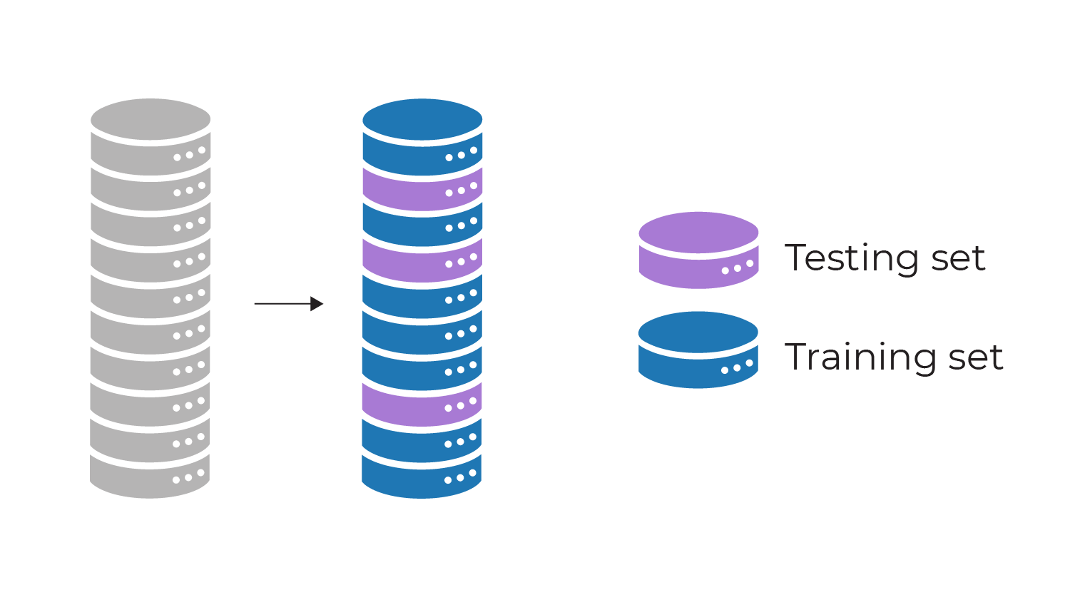You will have used code like this on several occasions:

# Split into train (2/3) and test (1/3) sets
test_size = 0.33
seed = 7
X_train, X_test, y_train, y_test = train_test_split(X, y, test_size=test_size, random_state=seed)

We build our model using the training set, but hold back the test set so we can evaluate the model using "unseen" data. This gives us an evaluation metric (the result of evaluating the model using the test set).

This testing using unseen data is the scientific method, which is key to being a good data scientist!

Here is a simple piece of Python code which loads the Boston house prices sample data set in preparation for building a machine learning model:

# Load Boston housing data set
boston = pd.read_csv("boston.csv")

# Define the X (input) and y (target) features
X = boston.drop("MEDV", axis=1)
y = boston["MEDV"]

# Rescale the input features
scaler = MinMaxScaler(feature_range=(0,1))
X = scaler.fit_transform(X)

And here is the code that builds a linear regression model and evaluates it using a train/test split, returning the R-squared score:

# Train test split
test_size = 0.33
seed = 7
X_train, X_test, y_train, y_test = train_test_split(X, y, test_size=test_size, random_state=seed)

# Create model
model = LinearRegression()

# Fit model
model.fit(X_train, y_train)

# Evaluate model
predictions = model.predict(X_test)
r2_score(y_test, predictions)

0.6663089606572572

Here is the workflow for the above code:

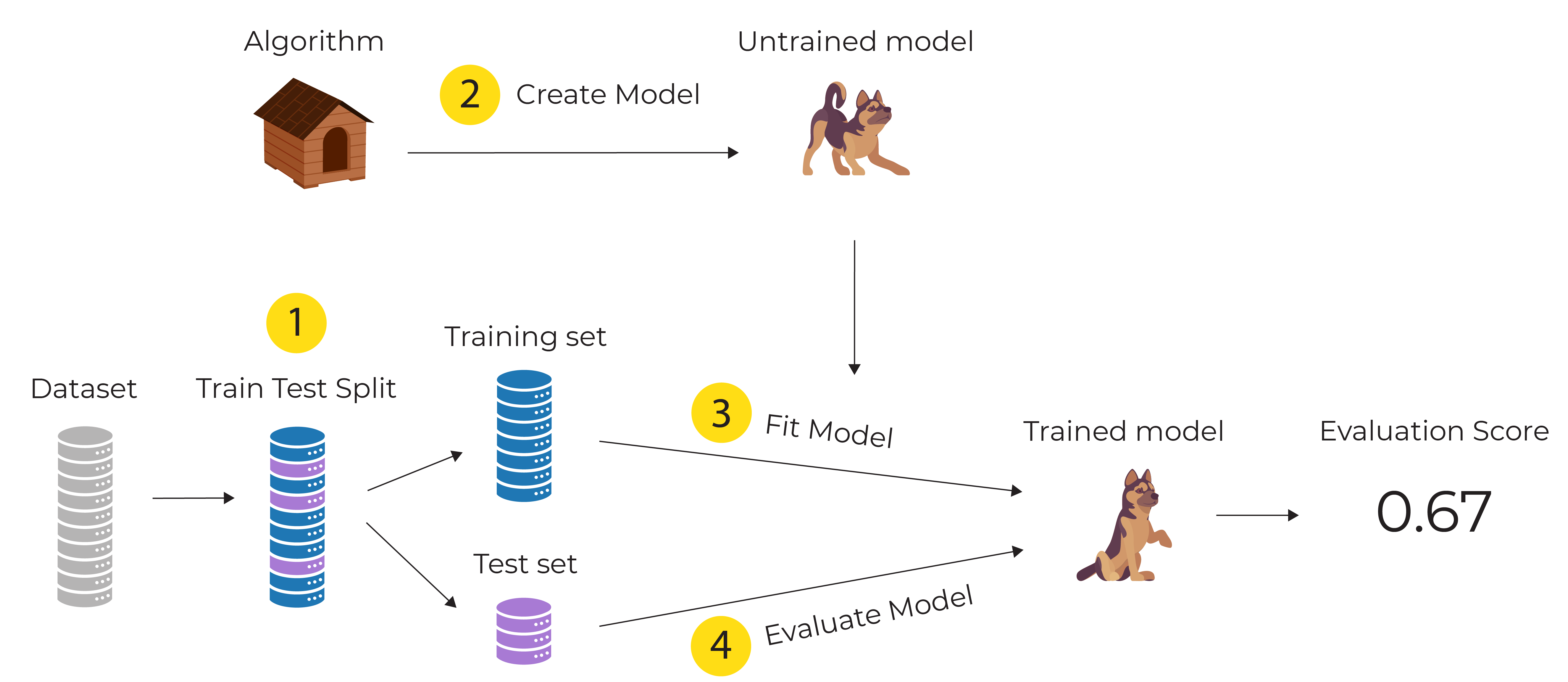
The steps are:

1. Split the data set into training and test sets based on random sampling (1/3 for test and 2/3 for training)

2. Take an algorithm and create a new untrained model

3. Fit the model using training data

4. Evaluate the trained model using test data

I could abbreviate the diagram for steps 2 to 4 like this:

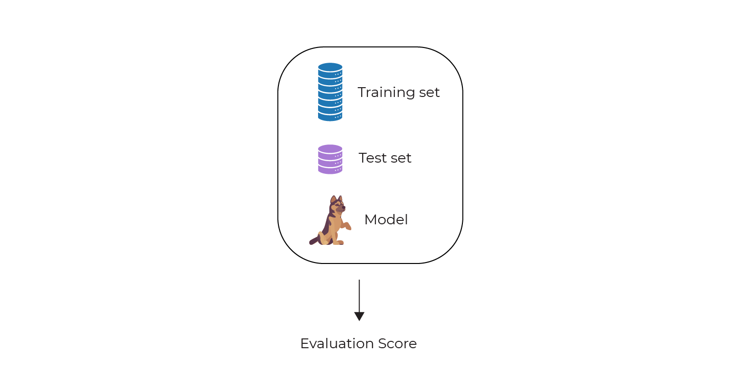
After running the above process we get an evaluation score for the model.

However, in your investigations, you may have observed that you get very different evaluation scores depending on the random seed chosen. The random seed determines the way the data is split by the train_test_split() function. There is a high variance in what falls into the training set and what falls into the test set with different random splits. This is not good, as it leads to inconsistency in the results and means we can't be confident in the evaluation scores we see.

In fact, cross-validation methods are used to provide a more robust evaluation of models. They work by splitting the dataset into multiple training and test sets and running the evaluation multiple times. Let's look at the most popular cross-validation technique...

Use K-fold Cross-Validation

K-fold cross-validation works by splitting the data into k subsets (called folds). Here we split into 5 folds:

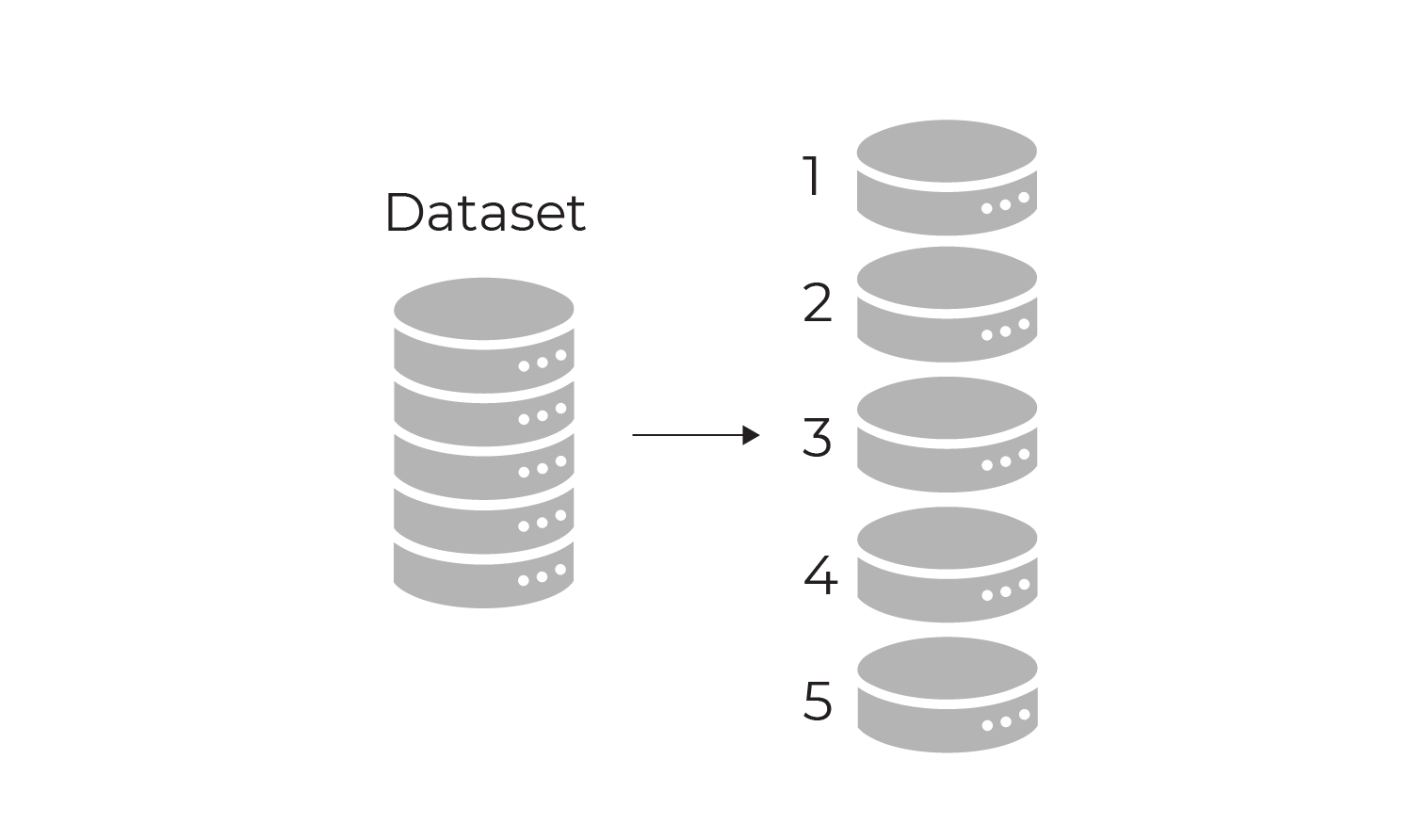
A model is trained using all but one of the folds. The model is then evaluated using the unused fold, which acts as the test set:

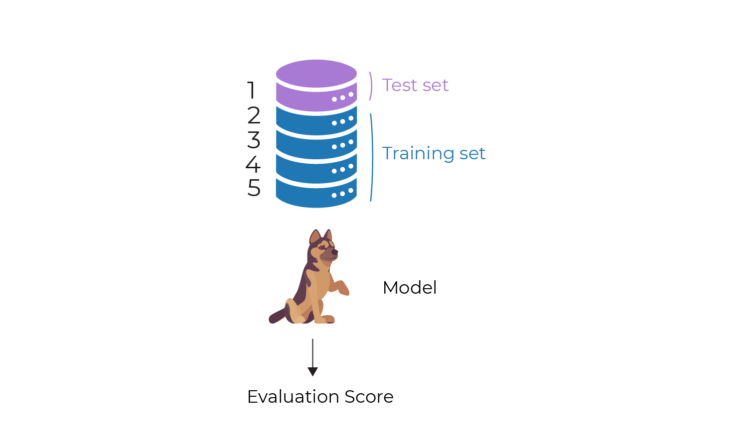
Diagram (b) above is carrying out exactly the same process as diagram (a) above. The only difference is that we have split the data into training and test sets in a different way.

This process is repeated, but keeping a different fold back as the test set each time. On completion, we will have trained and evaluated a model 5 times, and have 5 evaluation metrics.

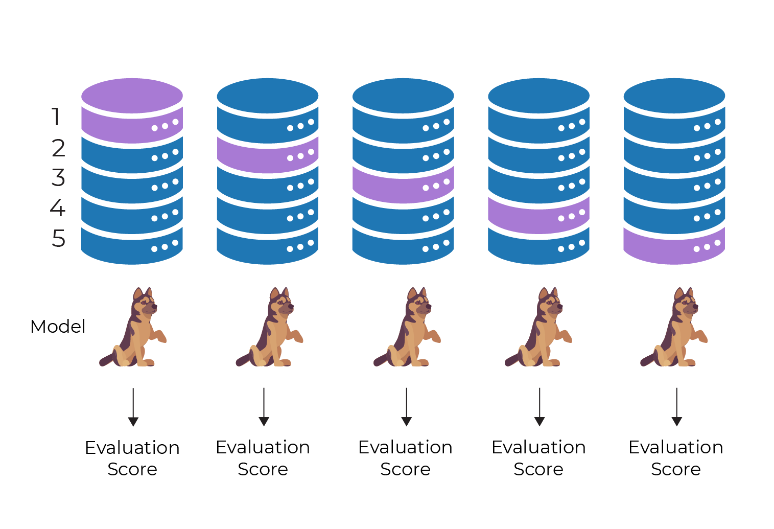
We can then compute an overall evaluation score by taking the mean of the 5 scores. In this way, we get a more robust evaluation of our models. They are less susceptible to being poorly evaluated due to the luck of the draw in the random sampling, because we've tested with 5 different cuts of the data.

We don't have to stick with 5 folds. Generally, somewhere between 5 and 10 will give you good results.

We can incorporate k-fold cross-validation very easily into our investigations using Sklearn.

# Create 5 folds
seed = 7
kfold = KFold(n_splits=5, shuffle=True, random_state=seed)

# Create a model 
model = LinearRegression()

# Train and evaluate multiple models using kfolds
results = cross_val_score(model, X, y, cv=kfold, scoring='r2')
print(results)
print("Mean:", results.mean())
print("Std:", results.std())

[0.57790144 0.76990344 0.64138006 0.73139225 0.80395154]
Mean: 0.7049057438479572
Std: 0.08354868173256094

The results list is the list of 5 R-squared scores, one for each of the k model evaluations. I've also shown the mean and standard deviation of these 5 scores, as a summary of the overall performance of linear regression across all 5 models. We can take the mean score (0.71) as our evaluation score for linear regression.

Here is the workflow for the above code:

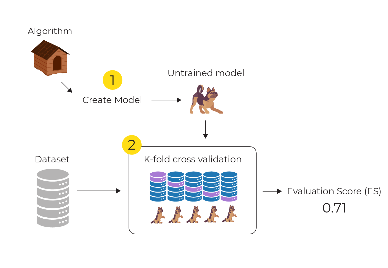
Note that we don't need to explicitly perform the train/test splits. The KFold object passed to the cross_val_score() function does this for us.

We can also get the predictions from the cross-validation analysis. Note that these are not actually model predictions as we are evaluating multiple models (one for each fold). Nevertheless, they can give a useful way of checking the potential real model predictions:

cross_val_predict(model, X, y, cv=kfold)

array([29.78263869, 25.18759152, 31.32588939, 28.58704763, 27.62169827,
25.8584904 , 22.75120309, 18.59873664, 10.76099096, 18.08494152,
18.51605175, 20.76908112, 20.48931998, 19.22031474, 19.44404476,
19.29017101, 20.39068546, 16.95335226, 17.63863428, 18.41757429,
...

The above example uses R-squared, but you can use different evaluation metrics. You can get a list of possible evaluation metrics (for both classification and regression) by running this code:

from sklearn.metrics import SCORERS
sorted(SCORERS.keys())

['accuracy',
'adjusted_mutual_info_score',
'adjusted_rand_score',
'average_precision',
'balanced_accuracy',
'brier_score_loss',
'completeness_score',
'explained_variance',
'f1',
'f1_macro',
'f1_micro',
'f1_samples',
'f1_weighted',
'fowlkes_mallows_score',
'homogeneity_score',
'mutual_info_score',
'neg_log_loss',
'neg_mean_absolute_error',
'neg_mean_squared_error',
'neg_mean_squared_log_error',
'neg_median_absolute_error',
'normalized_mutual_info_score',
'precision',
'precision_macro',
'precision_micro',
'precision_samples',
'precision_weighted',
'r2',
'recall',
'recall_macro',
'recall_micro',
'recall_samples',
'recall_weighted',
'roc_auc',
'v_measure_score']

Take a look at the sample code on the course GitHub repository for a fully worked example.

Summary

• When evaluating models, we should always evaluate using different data than that used to train the model. Resampling is used to separate training and test data.

• Train/test split splits the data into training and test sets. It trains the model with the training data and evaluates the model using the test data.

• K-folds cross-validation splits the data into k subsets and uses these to create multiple train/test sets. It takes each train/test set and trains the model with the training data and evaluates the model using the test data.

 In the next chapter, we are going to do some hyperparameter tuning!