Improve the Performance of a Machine Learning Model

As we saw early in this course, overfitting is the frequently-occurring enemy of the model-building data scientist! We've already seen a few ways to tackle this. In this chapter, we will look at regularization, a method to add control to our linear regression models.

Review Linear Regression

Remember our little friend, linear regression? :honte:

We keep coming back to this because it is so fundamental in a lot of machine learning. In this chapter, we will look at how to add a really useful control mechanism to linear regression, so we can fine-tune its behavior.

Remember that in linear regression, we take our training data (which we can think of as points on a scatter plot) and we find a line of best fit through the data. To compute how good a line we have, we can measure the distance from the training data points to the line. These distances are called residuals. Here is a linear regression line which attempts to predict happiness from income level. The training data are the blue points, the black line is the linear regression line, learned during training, and the red dotted lines are the residuals.

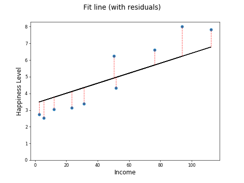
The residuals can be squared and summed, providing a measure called the Sum of Squared Residuals, or SSR. If $\$\backslash (y\backslash )\$$ is the true value for a point and $\$\backslash (\backslash hat\{y\}\backslash )\$$ is our linear regression prediction for the point, the residual for that point is $\$\backslash (y\; -\; \backslash hat\{y\}\backslash )\$$. So the sum of squared residuals is:

$\$\backslash [SSR\; =\; \backslash Sigma\; (y\; -\; \backslash hat\{y\})^2\backslash ]\$$

When training a model, the linear regression algorithm aims to minimize this function. It is called a loss function. Linear regression aims to minimize the loss, i.e. minimize the value of L in the following:

$\$\backslash [L\; =\; \backslash Sigma\; (y\; -\; \backslash hat\{y\})^2\backslash ]\$$

Review Overfitting

One problem you will encounter frequently in your machine learning journey is overfitting. We discussed overfitting earlier in this course. We saw that we can spot overfitting by ensuring we test our models in a proper, scientific way. We know when we have an overfit model. We get a much higher score on the training data than the test data. We also saw that selecting just a few good features rather than lots of features can help reduce overfitting.

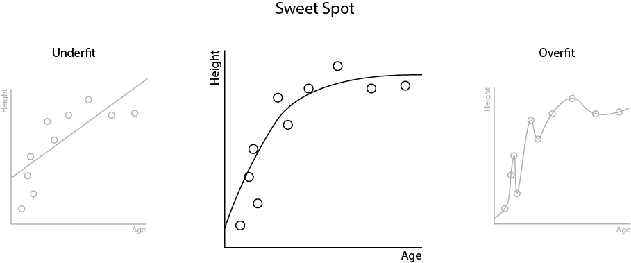
Overfitting results from having models that are too complex. Our aim in machine learning is to create the simplest models that describe the relationships in our data. But we don't want to make them too simple and swing the other way, towards underfitting. There is a sweet spot that we want to hit:

Use Regularization

Regularization adds a simple "lever" to our loss function. There are two variants:

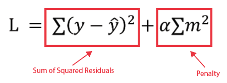
Ridge (L2) regularization modifies the loss function as follows:

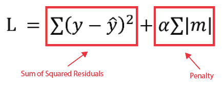
Lasso (L1) regularization modifies the loss function as follows:

In both cases, you can see that a penalty has been added to the SSR. The Greek letter $\$\backslash (\backslash alpha\backslash )\$$ (alpha) is the lever we can use to control the algorithm. Set it at 0 and the penalty disappears, so the loss function reverts back to plain old SSR and our model becomes plain old linear regression. But pulling the lever to increase alpha increases the overall penalty. 

The m in the above functions are the coefficients computed by linear regression. You will remember that the general formula for a linear regression line looks like this:

$\$\backslash (y\; =\; m\_1x\_1\; +\; m\_2x\_2\; +\; m\_3x\_3\; +\; ...\; +\; c\backslash )\$$

The $\$\backslash (m\backslash )\$$ s are the coefficients. They tell us how much influence each feature has on the target feature. For example, we may end up with a linear regression model for happiness that looks like this:

happiness = 2 * income + 3.3 * number_of_friends + 4.1 * number_of_pets - 5.6 * illness + 0.1 * your_football_team_win_ratio

The values 2, 3.3, 4.1 -5.6 and 0.1 are the coefficients. They tell us how much each feature contributes to predicting happiness. In attempting to minimize the loss function during training, Ridge and Lasso regression will have the effect of shrinking the magnitude of these coefficients. This will simplify the model, reducing overfitting.

You will see a slight difference between the Ridge and Lasso formulae above. Ridge sums the squares of the coefficients, whilst Lasso sums the absolute values of the coefficients. This drives slightly different behavior during training. Ridge drives coefficients towards zero, but they never reach 0. Lasso can drive the coefficients all the way to zero. A zero coefficient means the associated feature has no effect on the prediction of y. This means that Lasso can be used to eliminate features. 

For example, Lasso regression could drive the happiness formula coefficients down to:

happiness = 0.6 * income + 3.6 * number_of_friends + 3.9 * number_of_pets - 5.2 * illness + 0 * your_football_team_win_ratio

The feature 'your_football_team_win_ratio' has been eliminated, sacrificed in favor of more significant features.

Use Regularization in Python

Let's see how we can apply regularization in Python.

The code for this example can be found on the course Github repository.

Our example uses a modified version of the house prices data. You can find it in house_prices.csv on the Github repository.

Here is the code to load this data, apply feature scaling and split into X and y:

# Load the house prices data set
dataset = pd.read_csv("house_prices.csv")

# Split into X and y
y = dataset.SalesPrice
X = dataset.drop('SalesPrice', axis=1)
#X = X.loc[:, 'MS SubClass':'MS Zoning_RM']
X_dataset = X

# Rescale the input features
scaler = MinMaxScaler(feature_range=(0,1))
X = scaler.fit_transform(X)

# Train test split
test_size = 0.33
seed = 7
X_train, X_test, y_train, y_test = train_test_split(X, y, test_size=test_size, random_state=seed)

If we take a look at the data shape, we will see that there 305 columns:

dataset.shape

(2930, 305)

A lot of these columns are sparsely populated columns deriving from one-hot-encoded categorical features, such as the type of foundation or the quality of the kitchen. Take a look at the data to see this.

Let's build a standard linear regression model:

# Create model
model_lr = LinearRegression()

#Fit model
model_lr.fit(X_train, y_train)
predictions = model_lr.predict(X_train)
print("Train:", r2_score(y_train, predictions))

# Evaluate
predictions = model_lr.predict(X_test)
print("Test:", r2_score(y_test, predictions))

Train: 0.9383533342843932
Test: -8.417876639380045e+18

The R-squared score on the training data looks great, but the score on the test data is terrible! This is a sure sign that we have overfit the model.

Ridge Regression

Let's try the same with Ridge regression.

# Create model
model_r = Ridge(alpha=2)

#Fit model
model_r.fit(X_train, y_train)
predictions = model_r.predict(X_train)
print("Train:", r2_score(y_train, predictions))

# Evaluate
predictions = model_r.predict(X_test)
print("Test:", r2_score(y_test, predictions))

Train: 0.9251913512103855
Test: 0.880018158216308

That's a huge improvement in the R-square test score.

You will see that I chose an alpha of 2. How did I choose that? I guessed! But guessing is not a great approach and as you might expect, there is a better way to choose alpha. Alpha is just a hyperparameter, and in the previous chapter we saw how we can use grid search cross-validation to find the best setting for hyperparameters. Sklearn provides a dedicated function, RidgeCV() for cross-validation with Ridge regression. Here it is in action:

# Create 5 folds
seed = 13
kfold = KFold(n_splits=5, shuffle=True, random_state=seed)

# Create model
model_rcv = RidgeCV(cv=kfold)

#Fit model
model_rcv.fit(X_train, y_train)
predictions = model_rcv.predict(X_train)
print("Train:", r2_score(y_train, predictions))

# Evaluate
predictions = model_rcv.predict(X_test)
print("Test:", r2_score(y_test, predictions))

print("Alpha:", model_rcv.alpha_)

Train: 0.9060243584752139
Test: 0.8818617113087038
Alpha: 10.0

Cross-validation has determined that the best alpha for Ridge regression with this data is 10.

Lasso Regression

Let's do the same with Lasso regression:

# Create model
model_l = Lasso(alpha=1)

# Fit model
model_l.fit(X_train, y_train)
predictions = model_l.predict(X_train)
print("Train:", r2_score(y_train, predictions))

# Evaluate
predictions = model_l.predict(X_test)
print("Test:", r2_score(y_test, predictions))

Train: 0.9381307141916388
Test: 0.869940792687326

Again, we have some decent results.

Now let's try to optimize alpha using cross-validation:

# Create 5 folds
seed = 13
kfold = KFold(n_splits=5, shuffle=True, random_state=seed)

# Create model
model_lcv = LassoCV(cv=kfold)

# Fit model
model_lcv.fit(X_train, y_train)
predictions = model_lcv.predict(X_train)
print("Train:", r2_score(y_train, predictions))

# Evaluate
predictions = model_lcv.predict(X_test)
print("Test:", r2_score(y_test, predictions))

print("Alpha:", model_lcv.alpha_)

Train: 0.928377201303416
Test: 0.8816306830317462
Alpha: 51.88722443267619

We can see from the above that our objective in using regularization has been achieved. The improved test scores in relation to the training scores show that overfitting has been reduced significantly.

Visualise the Effect on the Coefficients

In the Jupyter notebook on the Github repository, I have included some code to visualize the coefficients in this example.

The following chart shows the 304 coefficients computed by the standard linear regression model. I've plotted these on a log scale as some of the coefficients were very large.

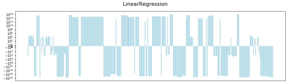
Note the scale on the y axis, from $\$\backslash (-10^\{18\}\backslash )\$$ to $\$\backslash (+10^\{18\}\backslash )\$$ .

Now here is the same using Ridge regularization with an alpha of 1:

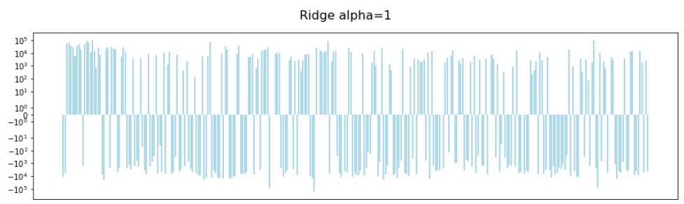
Note the scale on the y-axis has reduced to $\$\backslash (-10^\{5\}\backslash )\$$ to $\$\backslash (+10^\{5\}\backslash )\$$. We've had a big reduction in the magnitude of our coefficients.

Pulling the alpha lever up to 10 (the value chosen by cross-validation) gives us this:

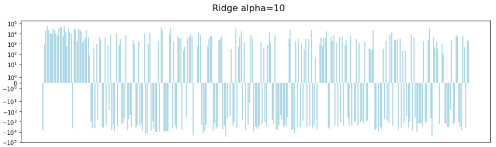
It's difficult the see, but the overall sum of the coefficients has reduced.

The impact of increasing alpha is more clear in Lasso regularization. Here we have an alpha of 1:

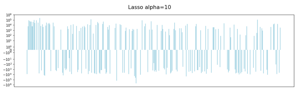
Increasing this to 50 (roughly the value chosen by cross-validation) gives us this:

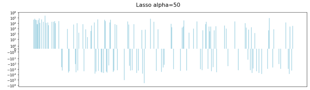
We can clearly see that some of the coefficients have disappeared. This is the in-built feature selection that Lasso brings.

Should I use Linear, Ridge or Lasso?

You now have three variants of linear regression at your disposal. So you may be wondering which to use. As always, the answer is "it depends". There is usually no clear up-front answer.

Lasso is useful where you have lots of features of varying significance and you want to do feature selection. Because it eliminates features, it also makes models more interpretable.

Ridge can perform better where you have a lot of features of roughly equal importance.

In practice, the best approach is to use experimentation with a number of techniques and cross-validation to see what works for your particular data.

Summary

• Linear regression can overfit, particularly where you have a lot of features.

• You can spot overfitting when you have a good training score, but a poor test score

• Regularization adds a penalty to drive the total magnitude of the coefficients down

• Ridge and Lasso regression have slightly different ways of doing this, and Lasso regression has the bonus of eliminating poorly performing features

 As this is the final chapter, I want to take a moment to thank you for taking this course! I hope that you now feel confident and dare I say, excited, to go off and evaluate and improve your machine learning models. Remember, practice, practice practice. Get hands on and try all the new techniques you have learned with some supervised models that you have built. And don't forget to take the final quiz of this course - it's yet another moment of practice! :magicien: Good Luck!