Introduction to Deep Learning Models

The goal of this part is to show you how a neuron works, and introduce you to neural networks. We will go from training a single neuron to training deep neural networks. Let's do it!

Your Task

You just came out of your very first briefing meeting! There seems to be an issue with how ingredients are passed down the conveyor belt. You are asked to use AI to fix that.

Here are some notes you took during the meeting to better understand how the ingredients are prepared and what the problem is:

• Ingredient Preparation Steps: Quality check→Washing→Sorting→Shipping

• Ingredients are all washed together (same line) 

• All items sorted by ingredient for packing/shipping to diff. franchises.

• Line splits into multiple different lines during sorting (1 line=1 ingredient)

• Problem=corn and olives often get confused on sorting line. Corn sneaks into the olive container, and vice versa.

• Cameras located above convey belts.

• Already have camera info. about shape+color.

• Action plan: Need to detect between corn and olives. Build model to detect each type of ingredient. 

Your colleague gives you information about what the data looks like:

You will have to load it into a pandas DataFrame, convert it into numbers so the machine can understand it, and then train an algorithm. Are you ready? Let’s do it!

Understand the Data

Start a new Jupyter Notebook and add the imports, you will use:

import pandas as pd
import matplotlib.pyplot as plt
%matplotlib inline

We will be doing some data manipulation here. If you find it hard to remember how to do them, this chapter about feature creation, entitled Create New Features from Existing Features, should help!

Load the data:

corn_and_olives_dataset = pd.DataFrame.from_dict({
        'shape': ['round', 'oval'],
        'color': ['yellow', 'green'],
        'ingredient_type': ['corn', 'olives']
    }
)

And check to see if it is correct:

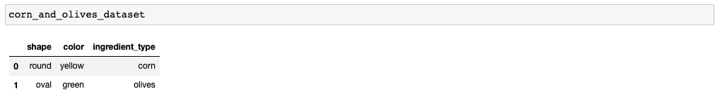
Next, convert the data from strings of 'yes' and 'no' to numbers - something the machine can understand:

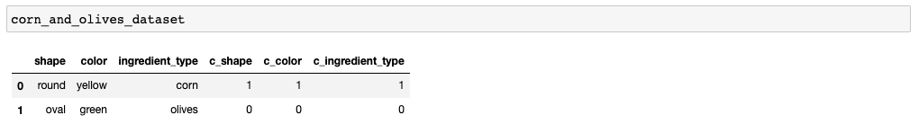
corn_and_olives_dataset['c_shape'] = corn_and_olives_dataset['shape'].apply(lambda x: 1 if x == 'round' else 0)
corn_and_olives_dataset['c_color'] = corn_and_olives_dataset['color'].apply(lambda x: 1 if x == 'yellow' else 0)
corn_and_olives_dataset['c_ingredient_type'] = corn_and_olives_dataset['ingredient_type'].apply(lambda x: 1 if x == 'corn' else 0)

The data should look like this now:

Let's see how the ingredients look on a plot:

corn_and_olives_dataset.plot(
    kind='scatter',
    x='c_shape',
    y='c_color',
    c='c_ingredient_type',
    colormap='jet'
)

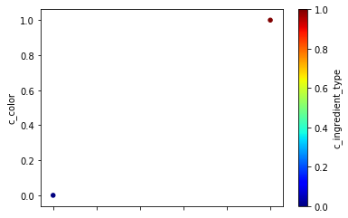
These two points can be separated by a single line running diagonally from the top left corner to the bottom right corner. Logistic regression, and more specifically, the sigmoid function can be used to separate these two points.

As you may observe on the graph, the function's output approaches 0 as the input becomes smaller and smaller. Inversely, it as the output's function approaches 1, the input gets larger:.

Let's set up the neuron to use exactly this function!

Set Up and Train Your First Neuron

You will be using three components to set up and train your neuron:

Component 1: The Network Structure 

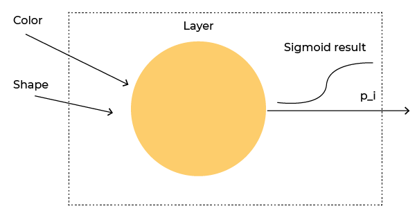
This sets up a neural network layer, which contains information about:

• The number of neurons,

• The number of inputs they require,

• And their activation function. 

Throughout this course, you will see different types of layers, but in this part, we will only work with dense layers.

That means that if the neuron is in the input layer of the network, it will see every column of the data. If it’s further inside the hidden layers, it will receive data from all the neurons in the layer before it.

Within a layer, a neuron first applies weights to the inputs when it needs to make a decision. Then, the neuron’s activation function decides how much it should fire based on these inputs and their weights. Just like a biological neuron! 

Let’s try adding a dense layer. Since this layer is an input layer, the neuron will receive all the columns of every data point:

from tensorflow.keras.layers import Dense

The layer setup is as follows:

• Units = 1; we only want one neuron for now. 

• Select 2 input dimensions - input_dim=2; we want to put through both color and shape.

• Sigmoid activation. 

from tensorflow.keras.layers import Dense

single_neuron_layer = Dense(
    units=1,
    input_dim=2,
    activation='sigmoid'
)

This is what you asked Keras to give you:

Behind the scenes, this is the neuron that Keras set up for you:

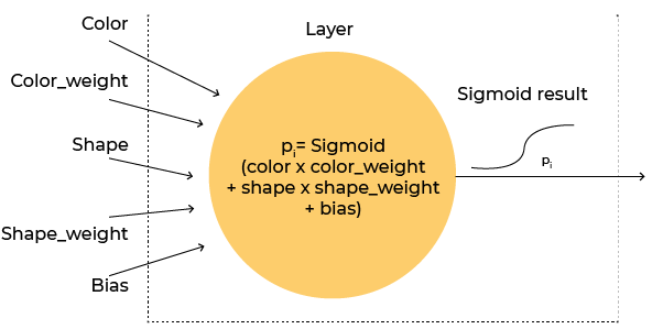
Keras has set up weights for every one of your inputs -colour_weightandshape_weight, as well as a bias term.

The weights and bias are the variables that will be modified during training to get as close as possible to the expected result.

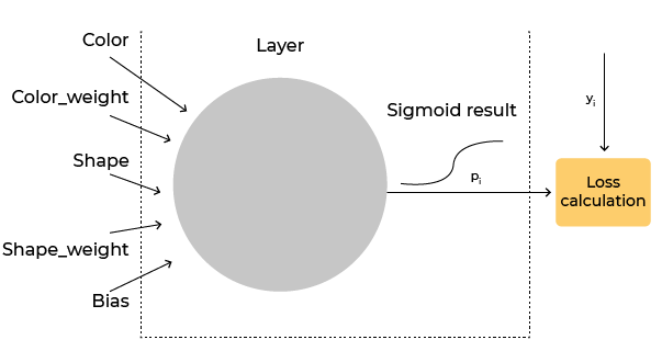
Component 2: Loss Function

This compares network results with expected results during training. These functions calculate the difference between what the network, or in this case, the neuron, outputs, and the value it should output. This difference is then used by the next component to tune the network to produce better results. They use the output from the neuron ( $\$\backslash (p\_i\; \backslash )\$$ ) together with the expected output ( $\$\backslash (y\_i\backslash )\$$ ):

One such function is binary cross-entropy. Binary cross-entropy (what we will use) looks at the difference between the two values - network output and expected output. Check it out below:

$\$\backslash [\backslash begin\{equation\}loss\; =\; y\_i\; *\; \backslash log(p\_i)\; +\; (1-y\_i)*\backslash log(1-p\_i)\backslash end\{equation\}\backslash ]\$$

Intuitively this equation has two types of results we are interested in:

1. The Loss Value Goes Up

If the output of the neuron and the expected value do not match, or are far apart, then the loss value goes up:

If the expected value is 1 -  $\$\backslash (y\_i\; =\; 1\backslash )\$$ and the neuron outputs a value close to 0 -  $\$\backslash (p\_i\; =\; 0.01\backslash )\$$  then:

$\$\backslash [\backslash begin\{equation\}\; loss\; =\; 1\; *\; \backslash log(0.01)\; +\; (1\; -\; 1)\; *\; \backslash log(1\; -\; 0.01)\backslash \backslash \; loss\; =\; 1\; *\; (-2)\; +\; 0\; \backslash \backslash \; loss\; =\; -2\; \backslash end\{equation\}\backslash ]\$$

Or the other way around if the expected value is 0 -   $\$\backslash (y\_i\; =\; 0\backslash )\$$  and the neuron outputs a value close to 1 -   $\$\backslash (p\_i\; =\; 0.99\backslash )\$$  then:

$\$\backslash [\backslash begin\{equation\}\; loss\; =\; 0\; *\; \backslash log(0.99)\; +\; (1\; -\; 0)\; *\; \backslash log(1\; -\; 0.99)\backslash \backslash \; loss\; =\; 0\; +\; 1\; *\; (-2)\; \backslash \backslash \; loss\; =\; -2\; \backslash end\{equation\}\backslash ]\$$

2. The Loss Value Goes Down

If the output of the neuron do not match, or are very close together, then the loss value goes down.

If the expected value is 1 -  $\$\backslash (y\_i\; =\; 1\backslash )\$$ and the neuron outputs a value close to 1 -  $\$\backslash (p\_i\; =\; 0.99\backslash )\$$  then: 

$\$\backslash [\backslash begin\{equation\}\; loss\; =\; 1\; *\; \backslash log(0.99)\; +\; (1\; -\; 1)\; *\; \backslash log(1\; -\; 0.99)\backslash \backslash \; loss\; =\; 1\; *\; (-0.004)\; +\; 0\; \backslash \backslash \; loss\; =\; -0.004\; \backslash end\{equation\}\backslash ]\$$

Or the other way around if the expected value is 0 -   $\$\backslash (y\_i\; =\; 0\backslash )\$$  and the neuron outputs a value close to 0 -   $\$\backslash (p\_i\; =\; 0.01\backslash )\$$   then: 

$\$\backslash [\backslash begin\{equation\}\; loss\; =\; 0\; *\; \backslash log(0.01)\; +\; (1\; -\; 0)\; *\; \backslash log(1\; -\; 0.01)\backslash \backslash \; loss\; =\; 0\; +\; 1\; *\; (-0.004)\; \backslash \backslash \; loss\; =\; -0.004\; \backslash end\{equation\}\backslash ]\$$

You can see that if the values are close together (network output 0 and neuron output 0 or network output 1 and neuron output 1), then the loss is minimal. As the values diverge, however, loss increases, penalizing the model.

loss='binary_crossentropy'

 Component 3: Optimization Algorithm

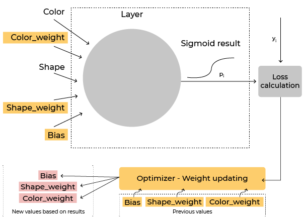
It does so by adjusting their weights and bias (in this casecolour_weight,shape_weight,  bias) to find the smallest loss value - the difference between the neurons' output ( $\$\backslash (p\_i\backslash )\$$ ) and their required output ( $\$\backslash (y\_i\backslash )\$$ ).

The loss looks something like the picture below. The network starts somewhere high on the curve (either left or right) and needs to find the weight value with a low error.

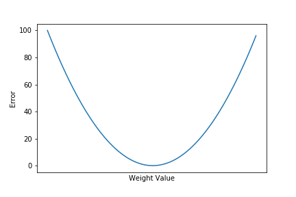
When adjusting the neurons' weights and biases, the optimization algorithm uses a learning rate parameter, which effectively tells it how big the adjustments should be. Large values for the learning rate translate as large adjustments, and smaller values translate as small adjustments.

A widespread optimization algorithm is stochastic gradient descent, which you will be using with the default learning rate:

from tensorflow.keras.optimizers import SGD
sgd = SGD()

Layers are connected sequentially, so that is how the model is set up:

from tensorflow.keras.models import Sequential
single_neuron_model = Sequential()

Finally, let's bring the components into the model and check out the setup using the  .summary()function:

single_neuron_model.add(single_neuron_layer)
single_neuron_model.compile(loss=loss, optimizer=sgd, metrics=[‘accuracy’])
single_neuron_model.summary()

Model: "sequential"
_________________________________________________________________
Layer (type)                 Output Shape              Param #
=================================================================
dense (Dense)                (None, 1)                 3
=================================================================
Total params: 3
Trainable params: 3
Non-trainable params: 0
_________________________________________________________________

You can see in the summary that we have a single neuron that outputs a single value, with three parameters to train (colour_weight,shape_weight,bias).

Use the  fit  function to train it:

history = single_neuron_model.fit(
corn_and_olives_dataset[['c_shape', 'c_color']].values,
corn_and_olives_dataset[['c_ingredient_type']].values,
epochs=2500)

Epochs refer to how many times the network should see the training data. In the code above, we said that we wanted the network to see it 2500 times.

In the last few epochs, you should be getting a loss similar to this or better:

Epoch 2497/2500
1/1 [==============================] - 0s 957us/step - loss: 0.1385 - accuracy: 1.0000
Epoch 2498/2500
1/1 [==============================] - 0s 1ms/step - loss: 0.1384 - accuracy: 1.0000
Epoch 2499/2500
1/1 [==============================] - 0s 1ms/step - loss: 0.1384 - accuracy: 1.0000
Epoch 2500/2500
1/1 [==============================] - 0s 945us/step - loss: 0.1383 - accuracy: 1.0000

Training is now complete. :soleil:

test_loss, test_acc = single_neuron_model.evaluate(
    corn_and_olives_dataset[['c_shape', 'c_color']],
    corn_and_olives_dataset['c_ingredient_type']
)

print(f"Evaluation result on Test Data : Loss = {test_loss}, accuracy = {test_acc}")

1/1 [==============================] - 0s 1ms/step - loss: 0.1551 - accuracy: 1.0000

Evaluation result on test data: Loss = 0.1550806164741516, accuracy = 1.0

Now, a single line can separate the data that represented the corn and olives.

Congratulations on training your first neuron! The factory is grateful for your help as they can now sort the ingredients automatically!

Let’s Recap!

• Neural networks contain three major components:

  • The network structure 

  • The loss function 

  • The optimizer

• The network structure defines the entire network and contains information about the number of layers, the number of neurons in each layer, and their activation function. The dense layer (where neurons receive every single feature of the data as input) is the most general type of layer. 

• Neurons work by summing the result of applying a weight to each input with a bias and then passing this result to an activation function tasked with producing the final result.

• When training, the loss function calculates the distance between the network’s result and the expected result. The optimizer then acts further to tune the network such that it can improve its results. It uses a learning rate parameter to know by how much to tune the networks’ parameters.

Now that you know how neurons work and how to build a small network let’s try to build a larger one in the next chapter!