Manipulate Rows and Columns

In this second part of the course, we’re going to get into the nitty-gritty! Keep your Excel document open so you can follow along. ;)
Now that you understand how cells work, let’s have a look at how to handle whole rows and columns.
Let’s take a look at the most common actions.
Insert and Delete Rows and Columns
To create a new column or row, you need to select the column or row that comes after it, then open the context menu and choose Insert.
For example, let’s say you want to insert a new column between “First Name” (column B) and “Last Name” (column C). You'd like this column to be named “Middle Name.”
Select column C (as this is the column you want to shift over to insert a column to the left) by clicking on the column heading, which is the letter C in this case.
Then right-click to open the context menu:
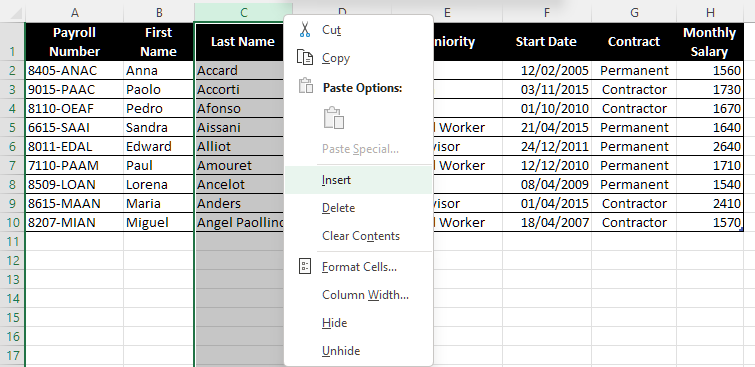
In this context menu, you just need to select the action you want to perform. In this case, Insert.
You now have an empty column that will be inserted to the left of the “Last Name” column.
Hide Rows and Columns
You’re going to use exactly the same method for this:
Select the row (or column) that you want to hide by clicking on its header (the letter for a column or the number for a row).
Open the context menu.
Select Hide.
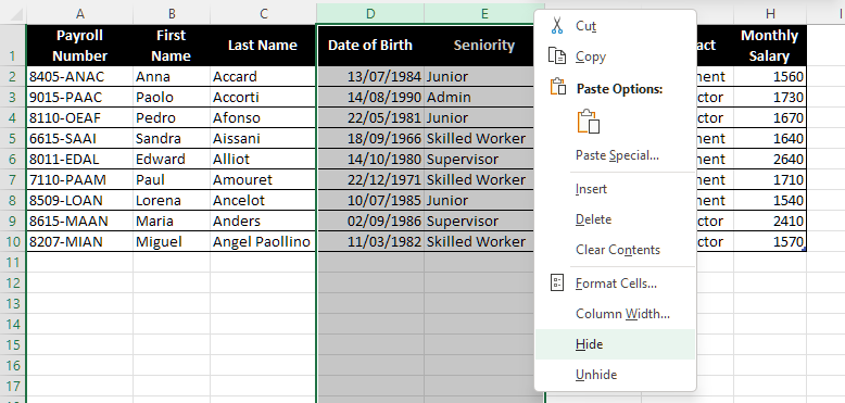
For example, in our file, maybe we don’t want the “Date of Birth” and “Seniority” columns to be visible, but you don’t want to delete them. In this case, you would select their respective columns, D and E, and choose “Hide” in the context menu.
The result will look like this:
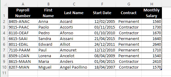
You can see that columns D and E (Date of Birth and Seniority) are no longer visible. But they haven't been deleted, it just skips from column C to F.
And if you want to make the hidden columns visible again:
Select columns C to F (i.e., include the columns either side of the hidden columns).
Open the context menu.
Select Unhide.
Columns D and E will then reappear.
Adjust Row and Column Sizes
You’ve probably noticed that when you enter data into a cell, some information overflows into the next cell.
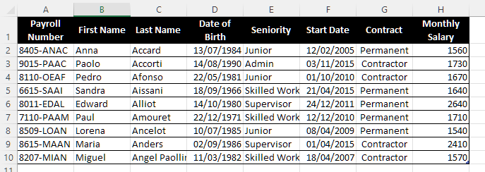
For example, in our file, Sandra’s seniority is quite long:
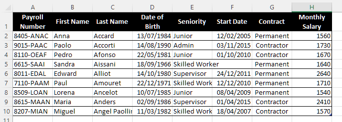
You can see that the seniority (cell E5) has overflowed because the column is too narrow. If you don’t make any changes, when you fill in cell F5, you won’t see the last part of the seniority:
If you want to avoid this, you can very easily change the size of the column. Or, more precisely, adjust it to fit the data that’s inside it.
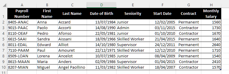
To do this, double-click on the separator marker between this column and the one next to it (in this case, the separator between E and F). The size of column E has automatically adjusted to fit the contents. This is also known as AutoFit.
You can also change the width of the column by clicking and dragging the column separator to adjust it however you’d like.
Group Rows and Columns
You might have a ton of columns that make your workbook hard to read, but you still need to retain the information inside them. One way to handle this is to group these columns together.
To group the columns, select the ones you’d like to group together, then in the Data tab, click on the Group icon  .
.
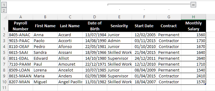
This is what you’ll see:
To hide grouped columns:
Either click on the minus (-) sign to hide the columns (which you can then unhide using the plus (+) sign).
Or, click on the 1 (and 2 to unhide).
It will then look like this:
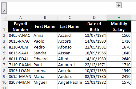
Columns E, F and G are hidden (but not deleted) and you see a plus (+) sign above the rows to indicate that the columns are grouped.
If you don't need to group the columns anymore and you don’t want the (+) and (-) signs above the columns, you’d need to ungroup the columns.
To ungroup the columns, select the columns that are grouped together, then in the Data tab, click on the Ungroup icon  .
.
Watch the Video Tutorial!
Watch a step-by-step recap of everything described in this chapter in the tutorial below:
Let’s Recap!
To insert a column, select the column heading to the right of where you want to insert it, then in the context menu, click on Insert.
To hide a column, select the column heading, then in the context menu, click on Hide.
To unhide a column, select the column headings either side of the hidden column, then in the context menu, click on Unhide.
To adjust the column width, double-click on the separator mark on the column heading.
To group columns, select the columns you’re interested in, then in the Data tab, click on the Group icon.
Now that you know how to handle rows and columns, let’s look at another feature in Excel: tabs.
