Table of contents
- Part 1
Use Basic Excel Functionalities
- Part 2
Work With Your Excel File
- Part 3
Manipulate Data in Excel
Table of contents
- Part 1
Use Basic Excel Functionalities
- Part 2
Work With Your Excel File
- Part 3
Manipulate Data in Excel
Create and Copy Formulas

Create and Copy a Simple Formula
Let’s imagine that you’re a store manager and you’re creating a sales tracking spreadsheet for a product.
In this sales spreadsheet, you've entered the first names of the sales staff and the number of items they’ve sold.
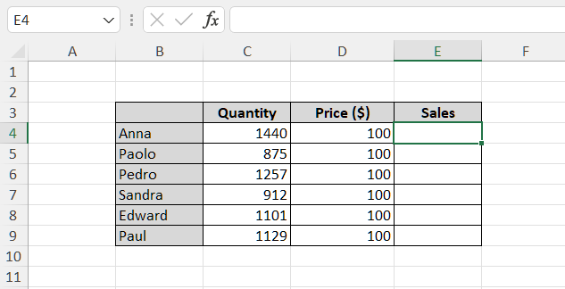
You’ve entered the prices of the items in cells D4 to D9, so now you want to calculate the sales figures (Sales in the workbook) for each salesperson, where Sales = Quantity x Price.
You're going to create a formula to calculate the result.
But this is the first time I’ve created a formula! 😱 I don’t know what I’m doing!
Don’t worry! You can create a formula very easily in just a few steps:
1. Select the destination cell, i.e., the cell where you want the result to appear. In this example, it's cell E4.
2. Type = . Formulas always start with the = sign.
3. Click on cell C4.
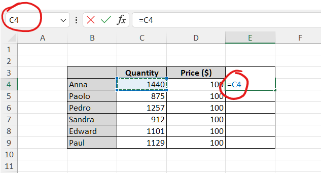
4. Type the * symbol on your keyboard (equivalent to a multiplication sign in Excel).
5. Select cell D4.
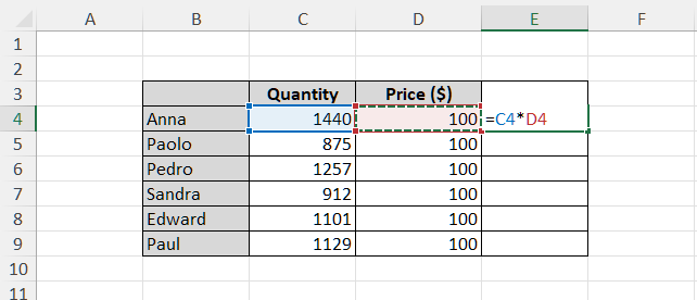
6. Hit the Enter key on your keyboard to confirm the formula.
And voilà—you've just created your first formula! 😃
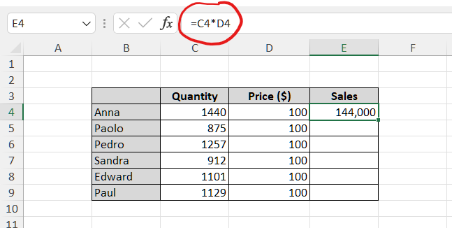
The result appears in cell E4 and the formula =C4*D4 appears in the formula bar.
Now you want to calculate the sales figures for the other salespeople without doing it all over again. You can copy cell E4 down to cell E9.
Let’s see what you get:
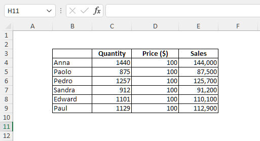
Now we’ll break down why this worked:
Take a look at this worksheet, which shows the formulas, not the results of the calculations.
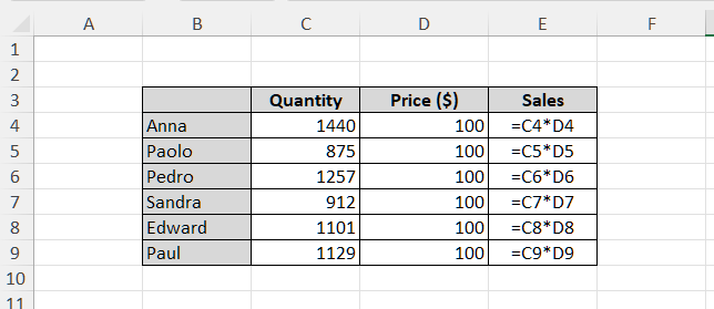
When you performed the fill series, the formula =C4*D4 was incremented down to the row below and became =C5*D5 and so on until the last one, =C9*D9.
Watch the Video Tutorial
Watch how to create and fill a simple formula step by step in the video below:
Create and Copy a Complex Formula
Don’t worry, this process is less complicated than it might seem! Let’s take the previous example. Given that the tracking sheet only shows one product, you decide to streamline it: instead of repeating the price several times in column D, you decide to calculate the sales figures after entering the price in cell D1.
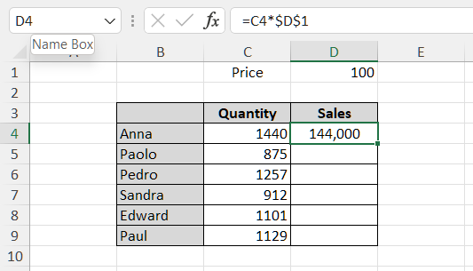
Now let’s build the formula that will allow you to calculate the sales figures:
Select destination cell D4.
To start your formula, type = on your keyboard.
Select cell C4.
Type * on your keyboard.
Select cell D1.
Confirm your formula with Enter.
After selecting cell D4, you can check the result below and you’ll notice that the formula appears in the formula bar.
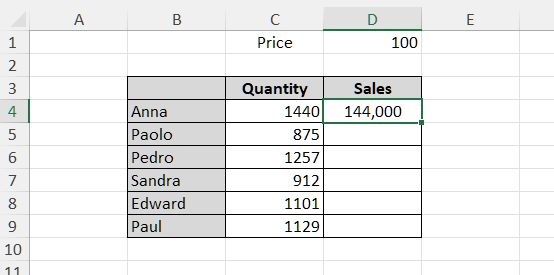
You're now going to copy cell D4 down to cell D9 and see what happens.
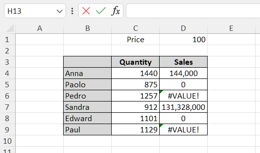
Oh no! Why didn't it work?
Take a look at this worksheet, which shows the formulas, not the results of the calculations.
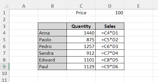
OK—let’s examine what happened. You used the fill handle to fill the series, and it did what it expected you to want: =C4*D1 changed in the next row below to =C5*D2 and so on, until the final entry =C9*D6. Not quite what you expected!
The formula =C5*D2 refers to cell D2, which is empty. And this also explains why the result in D6 is equal to #VALUE! Because the formula =C6*D3 refers to a cell that contains text.
Don’t worry, I can show you how to fix this!
In the example above, we’ve used what Excel calls relative references—references that change when a formula is copied. These are often very useful. However, we wanted the cell references to stay the same, so we need to use an absolute reference—a reference that remains the same, wherever it’s copied to. In this case, it will allow us to refer to cell D1 for all the formulas.
Now that we know this, let’s recalculate each salesperson’s sales figures:
Delete the results from D4 to D9.
Select destination cell D4.
To start your formula, type = on your keyboard.
Select cell C4.
Type * on your keyboard.
Select cell D1, which is currently a relative reference.
Once D1 is selected, press the F4 key on your keyboard and you’ll see the following result: $D$1.
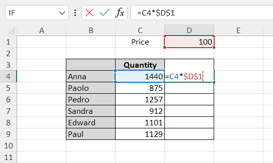
8. Hit Enter to confirm.
After selecting cell D4, you can see what happens below and check the formula in the formula bar.
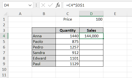
You're now going to copy cell D4 down to cell D9 and see what happens:
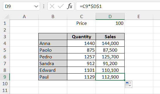
Now we’ll break down why this worked.
Take a look at this worksheet, which shows the formulas, not the results of the calculations.
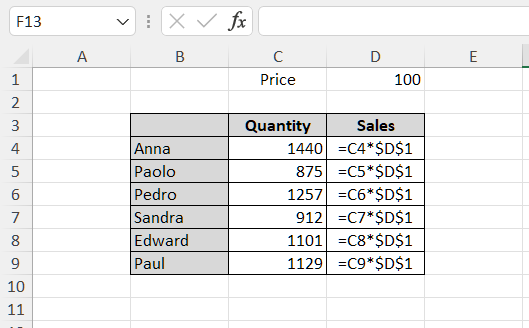
When you performed the fill series, cell C4 copied down to the row below and became C5 and so on until the last one, C9. However, all of the formulas now contain a constant cell reference that is recognizable by the use of the $.
In a fill series formula, the references are incremented automatically, except for the constant cell reference. We usually call these absolute references. If you’re a bit lost, don’t worry. All you need to understand for now is that if you copy a formula and you don’t get the results you were expecting, it might be because you should have used an absolute cell reference.
Get into the habit of asking yourself if you need to amend the references so that they are absolute, and remember that if you want to turn a relative reference, e.g., D1, into an absolute reference, you just need to press F4 or fn and F4 when the cell is selected. This will make the dollar signs appear in the cell to give us $D$1.
Watch the Video Tutorial
Recap the different steps required to create and fill a complex formula in the video below:
Let’s Recap!
You can create a simple formula to add, subtract, multiply or divide numerical values in your worksheets.
A formula is easy to spot, as it always starts with the = sign.
In a fill series formula, relative references are incremented automatically.
In a fill series formula, absolute references are not incremented.
To turn a relative reference into an absolute reference, you can use the F4 key or the fn key + F4.
You've now created your first formulas in Excel. Well done! Let’s meet in the next chapter and apply what you’ve learned in this first part of this course.
Ever considered an OpenClassrooms diploma?
- Up to 100% of your training program funded
- Flexible start date
- Career-focused projects
- Individual mentoring
Find the training program and funding option that suits you best
