Set up the Page layout

Now that you know how to adjust cells and tabs in Excel to your own specific needs, we’re going to look at the page layout.
Hide Gridlines
The gridlines you see on screen don’t appear when you print out the document. But to make your workbook more readable, you might want to hide the gridlines on screen as well.
It’s super simple to hide gridlines in an Excel tab:
Click on the View tab.
In the Show group, uncheck Gridlines.
As you've probably already worked out, if you want to show the gridlines again after hiding them, you do this in the same way by checking the Gridlines box.
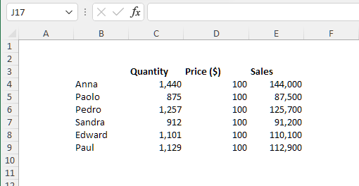
When the gridlines are hidden, you can no longer see the data boundaries for your worksheet. This could make it more difficult to read.
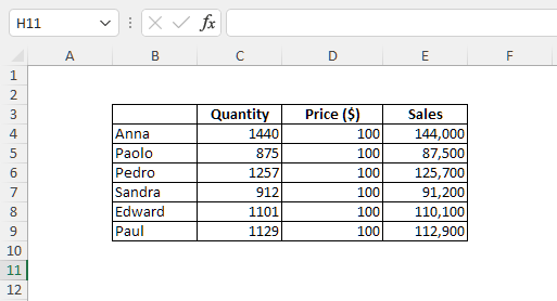
Let’s add some borders to make things clear:
Select the range of cells from B3 to E9.
Click on the Home tab.
In the Font group, click on the Borders icon
 .
.Select All borders.
Freeze Panes
Freezing panes is important when you're working on an Excel file that contains lots of rows or columns.
To avoid this problem, you can “freeze” panes, or keep the top row on screen visible even if you scroll down to the rows below.
To freeze panes:
Click on the View tab.
In the Window group, click on the Freeze Panes icon.
Select Freeze Top Row.
To unfreeze panes:
Click on the View tab.
In the Window group, click on the Freeze Panes icon.
Select Unfreeze Panes.
Wrap Cell Text
If you have lots of content within a cell, you can adjust the cell width to match the contents, as we saw in the chapter on rows and columns. But you could also wrap the text.
Here’s what that looks like (in this example, cells A1 and H1):
To wrap the text within a cell:
Select the cells whose contents you’d like to wrap.
Click on the Home tab.
In the Alignment group, click on the Wrap Text icon.
Watch the Video Tutorial!
Watch a step-by-step recap of everything described in this chapter in the tutorial below:
Print Your Workbook
Now you know how to set up the page in your file, you’ll be able to print it.
Print a Workbook
Click on the File tab.
On the sidebar, click on the Print command.
Click on the Print icon to trigger the print.
Print Titles
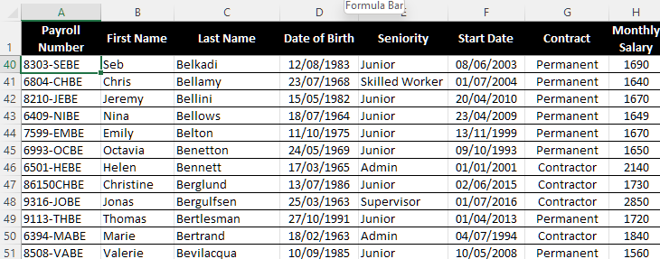
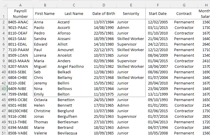
If your file is very big with lots of rows, it will be printed over several pages.
The column headings will be printed on the first page, but not on any of the following pages, which will make it difficult to read.
To avoid this, you can Print titles, which means repeat the column headings at the top of each page.
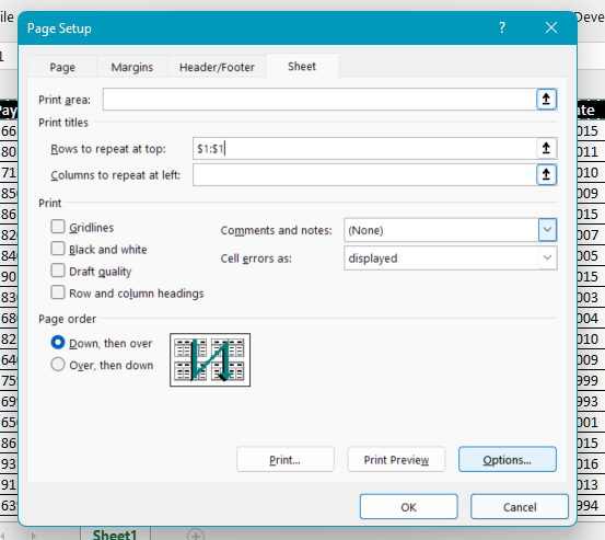
To print titles:
Click on the Page Layout tab.
In the Page Setup group, click on the Print titles icon.
In the Rows to repeat at top section, select the row in your worksheet that contains the headings.
Then click OK to confirm.
Add Page Numbers
When you want to print a file with several pages, you can ask Excel to add page numbers.
To do this, you can change the page footer.
To change the page footer:
Click on the Page Layout tab.
Click on the Page Setup button.
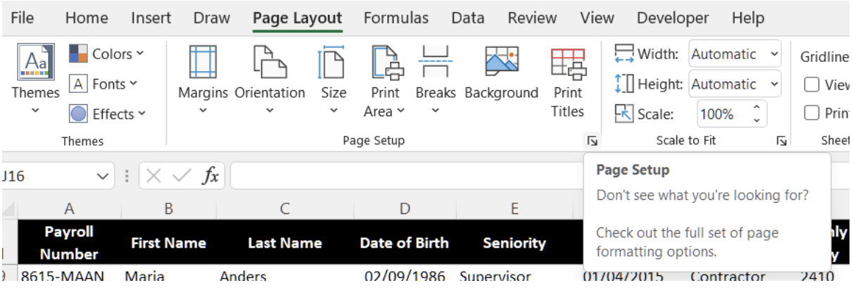
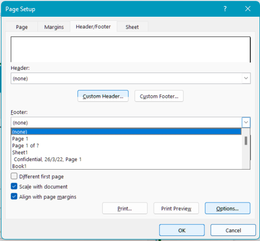
Go to the Page Setup dialog box.
Click on the Header/Footer tab.
In the Footer section, select Page 1.
Now, all your printed pages will be numbered.
Define a Print Area
When you’re working with a large file, you won’t always need to print the whole workbook. You can choose to print just part of it.
To do this, you can define a Print area.
To define a print area:
Select the area of the workbook that you’d like to print.
Click on the Page Layout tab.
In the Page Setup group, click on the Print Area icon
 .
.Select Set Print Area.
You’ll see that a black border has appeared to show you that a print area has been defined.
If you want to remove the print area:
Click on the Page Layout tab.
In the Page Setup group, click on the Print Area icon.
Select Clear Print Area.
Watch the Video Tutorial!
Watch a step-by-step recap of everything described in this chapter in the tutorial below:
Let’s Recap!
There are many page layout options within Excel. You can hide the gridlines, freeze panes and wrap text when a cell’s contents are too long to fit in the cell.
You can use different options to improve the look of your printouts, such as repeat headers over several pages, add page numbers and define a print area.
You now know how to set up your page layout and print your workbook. In the next chapter, we’re going to see how to format the page automatically using conditional formatting.
