Use Conditional Formatting

You now know how to set up your page layout and print your workbook. Let’s have a look at how to format your data automatically based on the contents of your cells.
For example, you might want the sales workbook to display amounts below $100,000 in red.
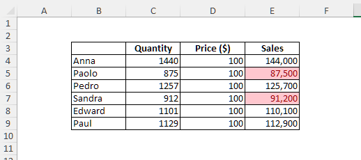
Of course, you could just change the color of the cells that meet the condition (less than $100,000), but if you did that and the figure was later increased to over $100,000, the cell would retain its formatting and stay red.
To avoid this, you’ll need to use conditional formatting.
To apply this conditional formatting:
Select the cells that you want to apply the conditional formatting to.
Click on the Home tab.
In the Styles group, click on the Conditional Formatting icon.
Select Highlight Cells Rules.
Then, click on Less Than…
This dialog box will appear:
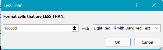
Click on OK to confirm.
By clicking on OK, the format that you've defined will be applied to all cells that meet the condition, i.e., where the amount is less than $100,000.
If you want to remove the conditional formatting:
Select the cells you want to apply the conditional formatting to.
Click on the Home tab.
In the Styles group, click on the Conditional Formatting icon.
Select Clear Rules.
Then click on Clear Rules from Selected Cells.
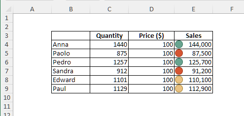
In the following example, you’re going to use three traffic light indicators based on each salesperson’s sales figures.
To apply this conditional formatting:
Select the cells you want to apply the conditional formatting to.
Click on the Home tab.
In the Styles group, click on the Conditional Formatting icon.
Select Icon Sets.
Within Shapes, select 3 Traffic Lights (unrimmed).
Conditional formatting is very useful for highlighting cells whose values meet a particular condition. It can be applied to a wide range of scenarios with many different options. The best way to discover all that conditional formatting has to offer is to play around with this feature on your own!
Watch the Video Tutorial!
Watch a step-by-step recap of everything described in this chapter in the tutorial below:
Let’s Recap!
Conditional formatting highlights values when a condition has been met.
You can create personalized formatting and specify your own conditions.
You can also use some of the many predefined formats that Excel has provided.
Conditional formatting is very useful for highlighting data that you want to draw attention to. It can be applied to a wide range of scenarios with many different options. Meet me in the next chapter to learn all about filtering and sorting.
