Table of contents
- Part 1
Use Basic Excel Functionalities
- Part 2
Work With Your Excel File
- Part 3
Manipulate Data in Excel
Table of contents
- Part 1
Use Basic Excel Functionalities
- Part 2
Work With Your Excel File
- Part 3
Manipulate Data in Excel
Use Filtering and Sorting Features

In this chapter, we’re going to cover two Excel features that help you to work more easily with large files with many rows and columns: filter and sort.
Filtering
How Filtering Works
When you filter your data, you’ll only see cells that meet the filter criteria, but the rest of the data won’t be deleted from the workbook, it will just be hidden.
Before we look at how to create a filter, here’s what it looks like.
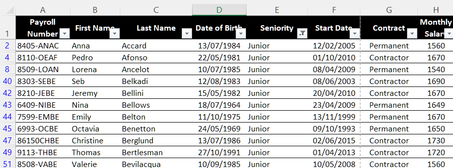
Here’s a workbook that only displays salary data for people with Junior in the seniority column (E):

You’ve probably noticed a couple of things:
The top row of this list with the column headings has a little downward arrow in the lower right corner. This means that filtering is currently active for this list.
The row numbers appear in blue and the funnel symbol in the Seniority column tells us that the list is currently filtered.
Now that you've seen what it looks like, let’s find out how to do it!
Create a Filter
To create a filter, follow these steps:
Select any cell in the list.
Click on the Home tab.
In the Editing group, click on the Sort and Filter icon.
Click on Filter.
You’ll see that an arrow will appear on each column heading.
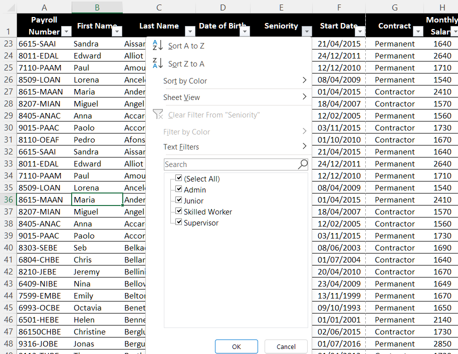
Click on the arrow on the “Seniority” column, and you’ll see this:

In the list that appears next to the Seniority column, you can:
“Select All” (by default), which means that all the data will be displayed and no filter is active.
check one or more levels of seniority that you want to be displayed.
check “Blanks” to only display cells with no data.
Use the Different Filter Rules
The three basic filter rules are number, text and color.
There are many filtering options:
Text filters, such as the one we used in our example.
Number filters, to display one or more value(s).
Date filters, to filter based on year.
From the 2016 version of Excel onwards, you can also filter by color.
Let’s take one last example for this chapter.
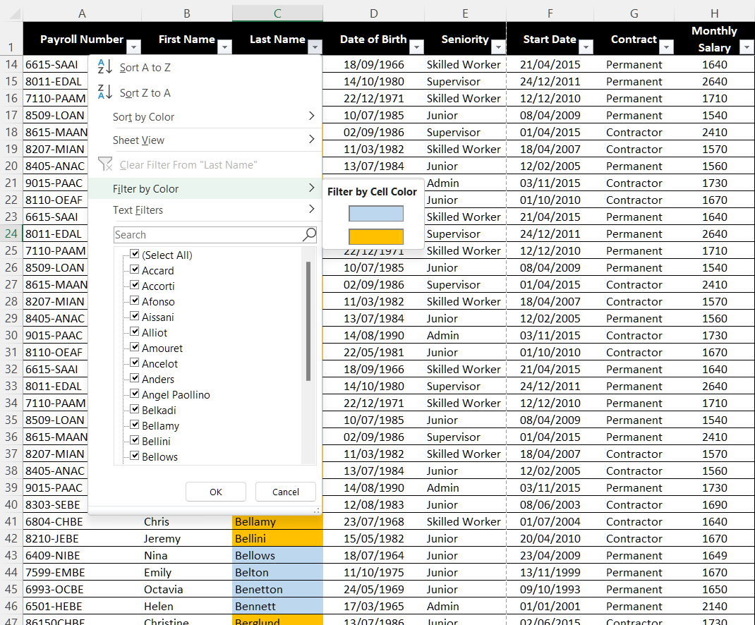
Let’s imagine that in your list of employees, you've colored the temporary employees or contractors in orange, and employees with permanent contracts in blue. If you activate the filter in the Last Name column, you’ll see this:

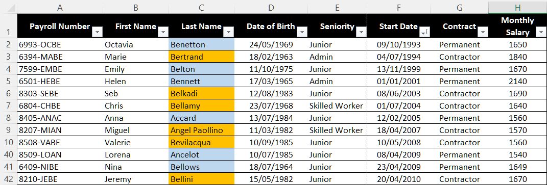
You can then select the color of the cells you want to display, which will hide the others.
Combine Several Filters
You can combine filters by filtering on several columns.
For example, if you only want to display employees with a seniority of “Skilled Worker” and who are working on a temporary basis, you need to:
Filter the “Seniority” column and select only “Skilled Worker.”
Filter the “Contract” column and select only “Contractor.”
You can combine as many filters as needed.
To turn off filtering:
Click on the Home tab.
In the Editing group, click on the Sort and Filter icon.
Click again on the Filter icon.
If you just want to reset all the filters:
Click on the Home tab.
In the Editing group, click on the Sort and Filter icon.
Click on the Clear icon.
Sorting
Before sorting the data, the cells are arranged in the order they were originally entered. The “sort” function allows you to change this, and works like this:
Select a cell in the column you want to sort by.
Click on the Home tab.
In the Editing group, click on the Sort and Filter icon.
Based on the type of data held in the column, you can sort:
from A to Z (Sort A to Z) for text fields.
from oldest (Sort Oldest to Newest) for date fields.
from smallest to largest (Sort Smallest to Largest) for numeric fields.

Watch the Video Tutorial!
Watch a step-by-step recap of everything described in this chapter in the tutorial below:
Let’s Recap!
Filtering enables you to display data from a list based on one or more criteria.
Data that doesn't meet the criteria is hidden.
Sorting data arranges it into a specific order.
You can sort using text, dates or numbers.
In this second part, you’ve seen how to set up the page layout for an Excel file, especially when you have lots of data. Now, let’s go and put what you’ve learned into practice in the next chapter.
Ever considered an OpenClassrooms diploma?
- Up to 100% of your training program funded
- Flexible start date
- Career-focused projects
- Individual mentoring
Find the training program and funding option that suits you best
