Create a Table

Your boss has received the file containing all sales data for Eastern Europe. You can download it here. Once you have deleted all unnecessary data, it’s time to move on to the data itself!
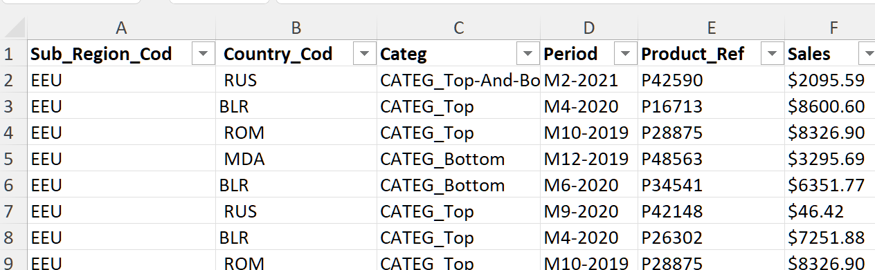
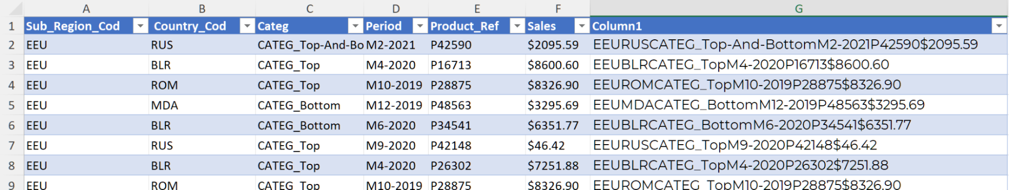
Here’s an extract of the file. It contains 1100 rows:
Prepare Your Data
Delete Unnecessary Spaces
You notice that some of the data in the list contains spaces that don’t need to be there, particularly in the “Country_Cod” field. These spaces mean that data inside the field does not have the same format, which makes it difficult for Excel to use this data.
You can use the TRIM() function to delete these spaces.
To use the function in this example:
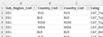
Insert a new column to the right of column B, then use this formula in C2: =TRIM(B2).
Use the drag handle to copy the formula up to cell C1116.
You’ll see that all of the unnecessary spaces before and after the cell value have disappeared.
You can now delete column B, as it is no longer needed.
The country codes are now usable. 😊
Find Duplicates
Create a Concatenation Column
Let’s start by creating a concatenation column. This puts all the information from a row into a single cell. You can then use this column to apply conditional formatting.
You’re going to use the CONCATENATE() function.
Insert the Concatenation Formula
Insert the following concatenation formula in cell G2: =CONCATENATE(A2,B2,C2,D2,E2,F2).
The result you get is “EEURUSCAT_Top-And-BottomM2-2021P42590$2095.59.” Granted, this doesn’t mean much, but that doesn’t matter too much here. 😁
Copy the Formula
Copy the formula all the way down to cell G1116, then copy and paste the results (using the paste function described in the previous chapter).
Select cells G2 to G1116.
Click on the “Conditional Formatting” icon, followed by the “New Rule” command.
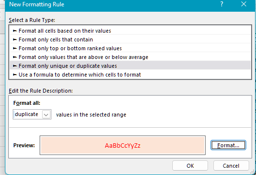
In the “New Formatting Rule” dialog box, select “Format only unique or duplicate values.”
Click on “Format” on the bottom right, and select a fill color and font. This formatting will be applied to any duplicate rows.
For example:
Click OK.
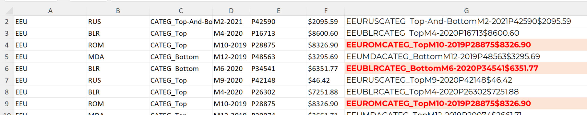
There are indeed some duplicate rows.
You’ll need to ask your boss what to do with these duplicates, so that you know whether or not to keep them.
Remove Duplicates
There are two ways of removing duplicates:
Either select the rows highlighted by the conditional formatting, and delete every other row... 😅
Or use Excel’s dedicated solution!
To remove duplicates efficiently:
Click on the “Data” tab, then on the “Remove Duplicates” icon
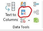 .
.Excel asks you to select the columns that you want to remove duplicates from:
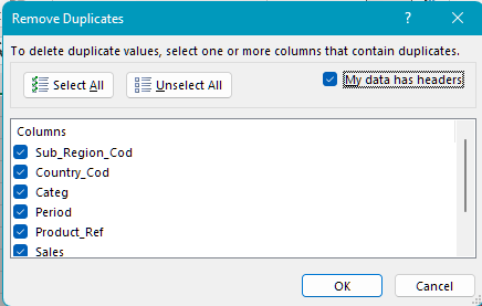
In this case, you want to remove fully duplicated rows, so you’ll need to check all the boxes.
Click OK, and a message will display telling you how many rows have been removed (without breaking it down further):
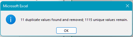
Your work is done!
Now check the “Concatenation” column (G), and you’ll see that the orange duplicate format has disappeared. 😊
Convert Your Data to a Table
Now that you’ve improved the quality of your data, you can convert it to an Excel table. 🥳
But what is the purpose of an Excel table?
When you enter data into a worksheet, Excel doesn’t know what you want to do with it. In this case, you know that you want to use a list of data provided by your boss, so you need to tell Excel!
This provides several advantages:
Excel will automatically add filters to your data columns.
A fill color will be applied to every other line, which makes the data easier to read.
If you add a calculated field, Excel will automatically apply your formula to the whole table.
If you add rows or columns to your table, Excel will automatically increase the size of the table.
To set up a table:
Select one cell from your current data. Click the “Insert” tab.
Under the “Table” group, click “Table”
 .
.Excel has a wide range of different styles and formats that you can choose from.
Excel asks you to confirm the cell area for your data:
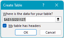
Click OK.
It might look something like this:
It already looks so much better! 😀 Transforming your data into a data table has other advantages, which we’ll cover later in the training program.
Over to You!
You have just received the full file for sales in Western Europe. You need to:
delete unnecessary spaces in columns B and D.
delete duplicate rows.
create an Excel table.
Answer Key
Check your work by downloading the answer key and watching the video below:
Let’s Recap!
Before using the data sources in your file:
Delete the unnecessary spaces.
Identify any duplicate rows, and remove them if required.
You can then transform your data list into an Excel data table.
You have now transformed the data from your source file into a data table. 🥳 Come with me to the next chapter, to find out how to adjust your table data to your requirements.
