Tailor Your Table to Your Needs

Now your data is in table format, you should ask yourself whether the data in its current form answers your boss’s questions.
You cannot use your data as it is. The categories are not clearly named, and both the “Period” field and the sales figures are in text format! 😕
Don’t worry! We’ll show you how to transform your data and make it usable. 😀
Tailor Your Text Data
Let’s start with a field containing text only, for example, the “Categ” field in column C of your table:
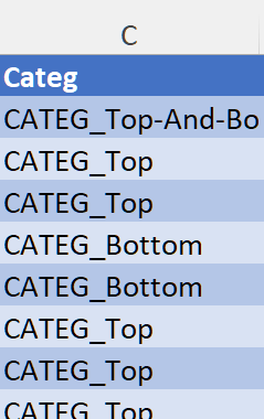
The objective here is to make the values easier to understand, by removing the “CAT_” text from the start of the data.
To achieve this, you’ll need to combine two “Text” category functions:
The RIGHT() function, because we need the right-hand part of the data
The LEN() function to count the number of characters in the cell, which can vary
How it works:
Insert two columns to the right of the “Categ” column.
The first, “Len,” counts the number of characters in the category.
The D2 formula is =LEN(C2).
The second, “Right,” extracts the right-hand part of the Categ column, taking all characters from the category minus six characters for the term “CATEG_”.
The E2 formula is =RIGHT(C2,D2-6).
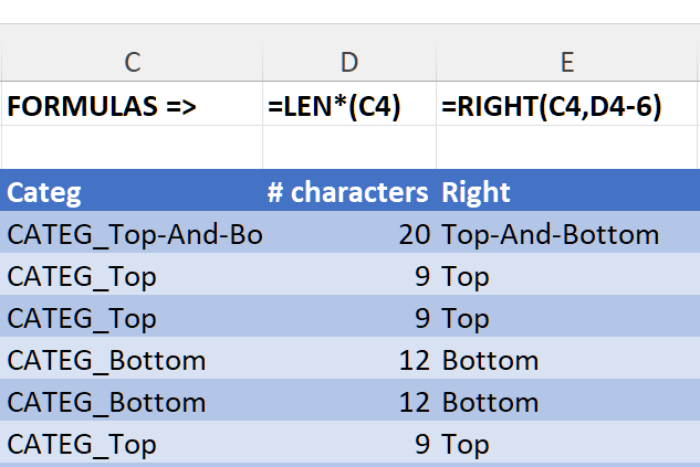
The data in the categories now makes sense.
Tailor Numerical Data
The sales data as shown cannot be used, as Excel is treating the data as text, because of the inclusion of the $ sign. You can tell this because
the cells are aligned to the left.
if you try performing any formulas on this column, you don’t get a meaningful response.
If you’re in doubt about whether data like this is in number format, there’s a simple formula you can try to demonstrate it.
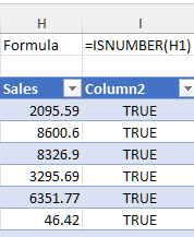
Create an empty column to the right of the Sales data in column H.
Enter the formula =ISNUMBER(H4) in cell I4.
The result will be either TRUE or FALSE… and you’ll know for sure!
So how can we fix this? It looks like it’s the $ sign that is confusing Excel, so we need to remove it. The simplest way to solve that is this.
Select the whole of column H.
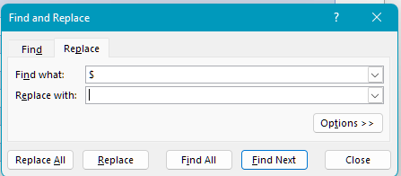
In the ‘Home’ ribbon, click on Find and Replace
 and select ‘Replace.’
In the ‘Find what’ box, type the dollar sign ($).
Leave the ‘Replace with’ box blank.
Hit ‘Replace All.’
The value in your ‘ISNUMBER’ column will now be TRUE… You can delete Column I, and you are now working with useful numerical data!
Use NUMBERVALUE
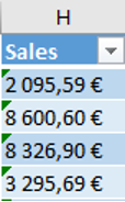
Another way that this problem can be resolved is to use the VALUE or the NUMBERVALUE command. These commands are particularly useful if your values in the Sales column are in a currency other than US Dollars or British Pounds—such as Euros, as in the example here.
The cells are aligned to the left.
The cells contain a comment (little green triangle) indicating that the format is wrong.
Luckily, you can transform the number from text format to number format, using the NUMBERVALUE() function.
To do so:
type the following formula into cell G2 =NUMBERVALUE(F2, “,”).
Excel transforms the data into a number.
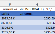
Excel has transformed the data into a number using the VALUE() function
You’ll see that the data is now aligned to the right, which Excel does with all numerical values.
Tailor Date Data
You may also have noticed that the “Period” column contains dates that are unusable:
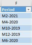
The aim here is to transform data into dates using the “01/01/2020” format, which Excel can use.
To do so, you’ll need five functions:
The LEFT() function, which you can use to get the year and isolate the month.
This tutorial will show you how to use it with the fx wizard!
The RIGHT() function and the LEN() function, which will also help you to extract the month number.
The FIND() function, which finds the hyphen location in the cell.
Finally, the DATE() function, which combines all four of the above functions.
This is a two-step process:
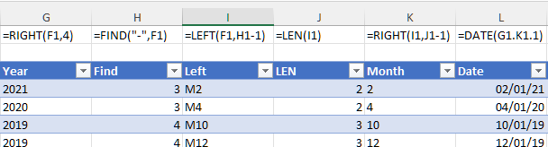
1. Insert Six Columns to the Right of the “Period” Column
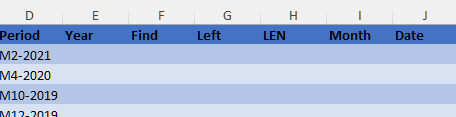
Column 1, named “Year”:
Isolates the year
Formula =RIGHT(D2,4)
Column 2, named “Find”:
Isolates the location of the hyphen
Formula =FIND(“-”,D2)
Column 3, named “Left”:
Isolates the month, including the letter M
Formula =LEFT(D2,F2-1). Here, you deduct 1 from H2, as H2 indicates the location of the hyphen, which is one character after the month.
Column 4, named “LEN”:
Counts the number of characters in column 3
Formula =LEN(G2)
Column 5, named “Month”:
Isolates the month number without the “M” (by deducting 1 from the total number of characters in column 4)
Formula =RIGHT(G2,H2-1)
Column 6, “Date”:
Creates a date using the year and month number from previous columns
Formula: =DATE(E2,I2,1)
You should get the result below:
2. Change the Cell Format
Using the correctly formatted date (Date field), you can now change the cell format to display the month:
Select column L, “Date.”
Right-click to display the context menu, then click “Format Cells.”
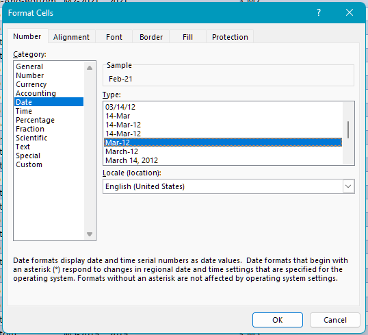
The column now displays in the correct format:
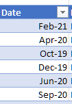
Ta-da! Excel now understands that this field contains dates! 😉
Over to You!
Your table contains data that Excel can’t use. To resolve this:
“Categ” column: remove characters on the left up to the hyphen.
Transform the “Period” column into dates that Excel can use.
Transform the “Sales” column into numbers that Excel can use.
Answer Key
You can find the answer key here and watch the video below to check your work.
Let’s Recap!
Manipulate text cells using the LEFT(), RIGHT(), and LEN() functions.
Transform the number from text format to number format, using the VALUE() function.
Transform a date from text format into date format, using the DATE() function.
The data in your table is now usable! You’ll still need to enhance this data to achieve your goal! Join me in the next chapter to find out how!
