Enter Advanced Formulas

You have your data, and your model is ready to populate. It’s time to let your data do the talking! 😊
Please download this file so that you can follow the various steps in this chapter. This file will serve as our starting point.
Use Complex Filters
You want to answer the following question for the region as a whole:
“Are the 2018 collection pants selling as well as the 2020 collection ones?”
You’re going to use complex filters to find the answer. There are a number of steps that you’ll need to go through.
Create the Criteria Range for the Complex Filter
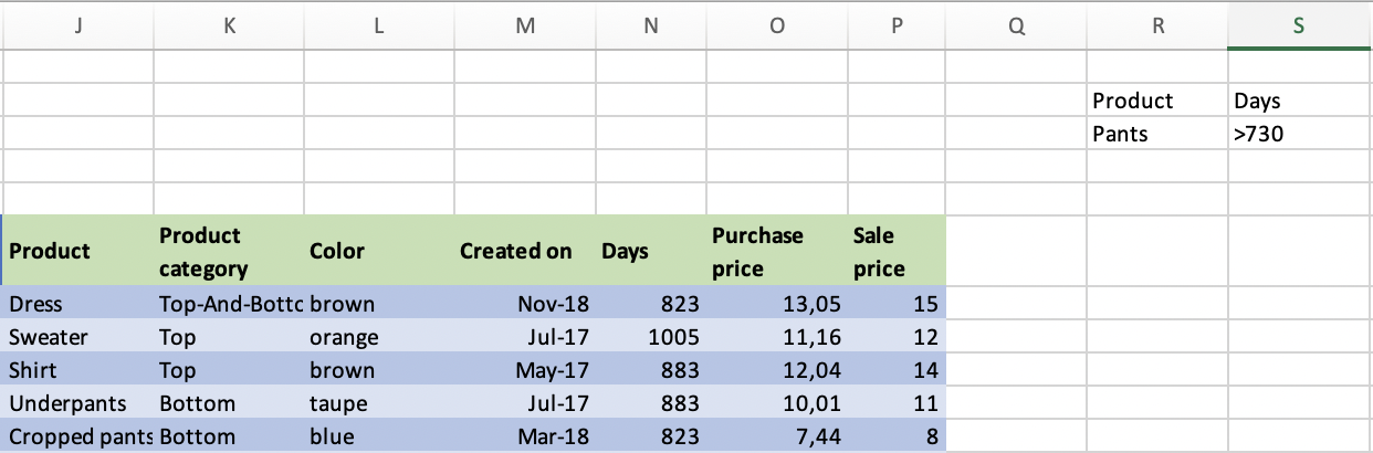
The criteria range is a cell range containing filters to be applied to the table.
Insert five new rows above the table.
Type out the column names that you want to filter to the top right of the table. In this case, they are “Product” and “Days” in R2 and S2.
Under “Product,” enter “Pants,” and under “Days,” enter “>730,” to get sales of pants created two years ago or more (730 = 365 days x 2).
Filter Your Data Table
Now the criteria are ready, you can filter your table:
Select a cell in your table.
Click on the “Data” tab, “Sort & Filter” group, then “Advanced.”
In the dialog box which opens, check the data range and enter the criteria range as R2 to S3.
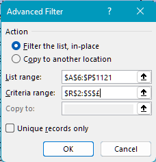
Click OK.
The data table has now been filtered on all pants created two years ago or more.
The result contains 49 rows! 😊
On the bottom left of your screen, you’ll see the number of filtered records:

Change Filter Criteria
Filter criteria combine two filters:
The database is filtered on the product “Pants.”
Within this selection, the second criterion filters days based on “>730.”
The criteria can be described as being added, using the condition “AND.”
You can modify these criteria to obtain an “OR” condition, which means:
I am filtering the database for the product “Pants.”
And:
I am adding rows with “>730” days (whether or not the product is “Pants”).
To create this new criterion, you’ll need to make the following changes to the filter range:
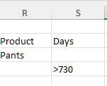
Each criterion is now on a different line!
If you re-run your complex filter with these new criteria, you’ll get 734 lines of results! 😀
Calculate Simple Statistics
Name a Cell Range
Excel lets you name a cell or cell range. This really helps to make your formulas easier to understand.
To name cells in the starting point file table:
Select the cells from the table.
Enter a name with no spaces or special characters (apart from “_”) into the Name box, to the left of the formula bar. In this example, the name is “Named_Range.”
Confirm by hitting the Enter key.
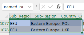
From now on, as soon as you use this name (either in the Name box or in an Excel formula), Excel will know that you’re referring to this cell range!
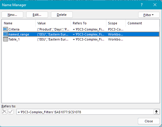
In this example, the name “Named_Range” has a range reference: =Table13468911127[#All].
This reference refers to all cells in the table, hence the name. If you had named the cells D2:B3 “my_range,” the reference would have been ='P3C2-Complex filters'!$D$2:$D$3.
Use Database Functions
Now that you know how to name a cell range, don’t forget to make use of this skill! The aim is to calculate simple sales statistics, so that you can answer the question “How have our Western European sales been going since 2019, by garment and on a quarterly basis?”
Follow the steps to use this function:
Enter the criteria to the right of the table. In R2, enter “Year-Quarter” with the value “2019-Q2” below, and “Category” in S2, with the value “Top” below.
Note that the labels and the format of the values have to be an exact match with what’s shown in the table itself!
Type the DSUM() function into S5, as follows: DSUM (Range_Name,“Sales”,R2:S3)
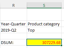
The range name makes the formula really easy to read.
You can also modify the criteria manually so that the formula updates automatically.
Calculate Conditional Statistics
Calculate Using Functions Based on a Sole Condition
The Dxxx() functions work well, but they require criteria cells to work, which means that they are sometimes difficult to manage if you have a lot of them.
Excel offers other solutions for producing simple statistics, including the SUMIF() formula, which is often used as it is very easy to read.
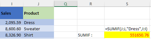
By way of example, we want to calculate total dress sales in the file. The SUMIF() function contains three arguments:
The column in the table which contains the criteria, in this case, products (column J)
The name of the relevant criterion, in this case, dresses
The column to which the sum applies, in this case, sales (column I)
The function therefore looks like this: =SUMIF(J:J,“Dress”,I:I).
Calculate Using Multiple Condition Functions
If you want to combine several criteria without using the criteria cells, Excel has created a few functions, which are recognizable due to the “S” added to the end.
The SUMIFS Function
You are going to use the SUMIFS() function to analyze sales by quarter and by category. This function works in the same way as the SUMIF() function, but you can add as many criteria as you want. The number of arguments varies based on how many criteria you need.
The syntax is as follows:
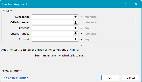
The first argument (“Sum_range”) is where the sum goes.
The second argument (“Criteria_range1”) is paired with the third argument (“Criteria 1”).
The third argument (“Criteria_range2”) is paired with the fourth argument (“Criteria 2”).
Using This Formula
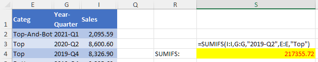
In our example, in cell T4 the formula is written as: =SUMIFS(I:I,G:G,“2019-Q2”,E:E,“Top”).
Using This Formula in Our Practical Example
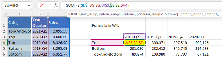
In our two-criteria example, it is easiest to create a double-entry table, and to create a formula which uses both the row and column names!
Using absolute references and the $ symbol, you can make sure that Criterion 1 matches the rows, while Criterion 2 matches the columns.
This is what the formula looks like in cell V4:
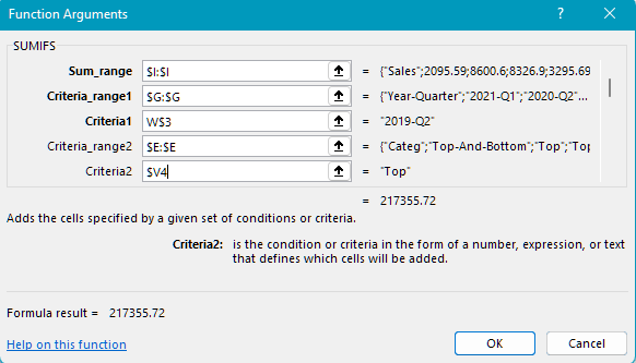
For cell W4, the arguments window looks like this:
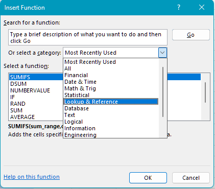
Use Predefined Functions in Excel
Excel has predefined functions for different business sectors, including financial, statistical, accounting and real estate.
Over to You!
Download this file and do the following:
Use a complex filter to count the number of rows which contain sock sales for France.
Create a data range called “My_DB,” which refers to the entire data table.
Count the number of rows of orange pants sales in June 2019, using the DCOUNTA() function, by re-using the “My_DB” name that you have just created.
Use the SUMIFS() function to calculate total green dress sales.
Answer Key
Look at the answer key and watch the video below to check your work.
Let’s Recap!
Use complex filters to filter your table based on several criteria.
Use the SUMIF() and COUNTIF() functions to calculate simple statistics based on one criterion.
Use the SUMIFS() and DSUM() functions to calculate statistics based on several criteria at the same time.
Your table now contains advanced formulas. Join me in the next chapter to find out how to tailor nested formulas to your own needs.
