Perfect Your Excel Skills

Tailor Formulas to Your Needs

You now know how to find functions which meet your requirements. Unfortunately, none of them meets your specific needs. 😕

Don’t worry. There is always a way, which most often involves combining different functions. 😉

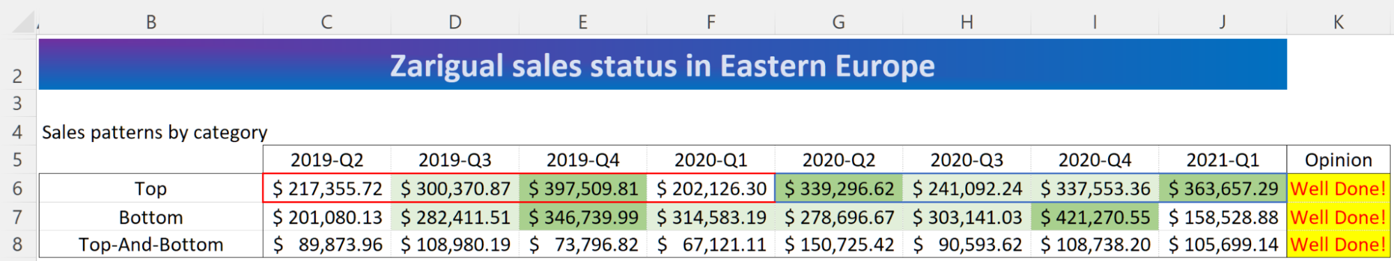
Download this file which contains sales from your dashboard.

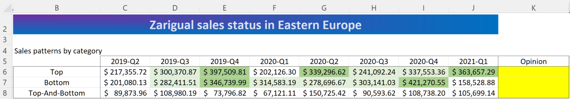
You need to use this data to give your opinion, based on a number of criteria:

• If sales from the last four quarters are higher than the four previous quarters, you display “Well done!”

• If not, you display a hyphen (“-”).

Excel doesn’t seem to have a function which will provide this result, so it’s down to you to build one! 😅 In this case, you’ll need to combine the functions IF() and SUM() by following several steps:

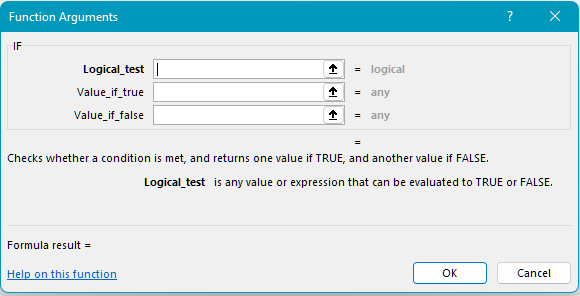
Define the Condition

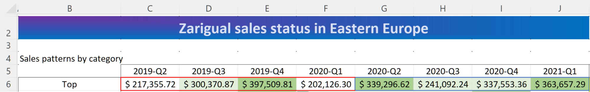
The condition for the IF() function is shown in the image below:

Select the Main Function

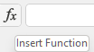
Using the “fx” icon:

• Click on the “fx” icon to the left of the formula bar, which opens the “Insert Function” tool .

• Look for the IF() function in the list.

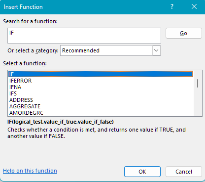
• Click “OK.”

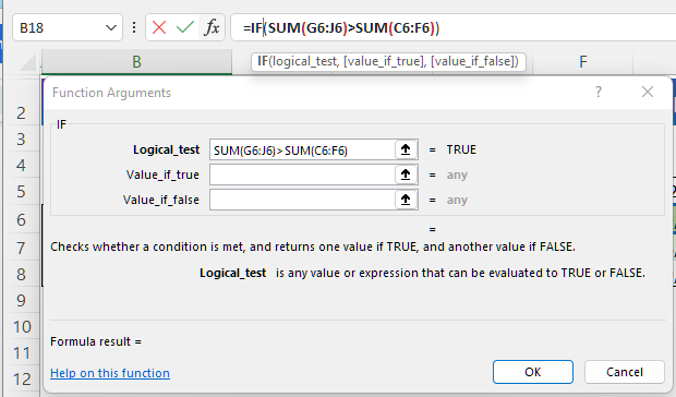
• Excel displays the arguments selection window.

In the “Logical_test” field, instead of entering a value, you want to enter a calculation for the gap between last year’s sales and the sales of the previous year.

• Click in the “Logical_test” field.

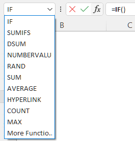
• Click on the name box to the left of the formula bar. This box now displays a list of Excel functions.

Select the Secondary Function

This is where you select the nested function, in this case SUM().

• Click on “SUM.”

• Excel displays the SUM() arguments window.

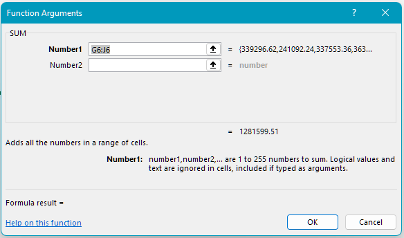
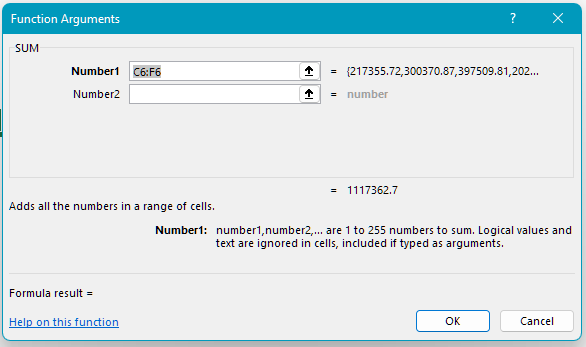
• Select the cells for the last four quarters, in this case, G6:J6.

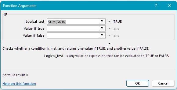
• Click on the “IF” text in the formula bar to go back to the IF() function arguments window.

Go back to the IF() function arguments window, which now contains the SUM() function as the first argument.

• In the “Logical_test” field, enter “>” to make the comparison between last year and the previous year.

• Click in the name box again to add the second sum, for the previous year.

• Now select the C6:F6 cell range.

• Click on the “IF” text on the formula bar to go back to the IF() arguments window.

• In the “Value_if_true” field, enter “Well done!”

• In the “Value_if_false” field, enter “-.”

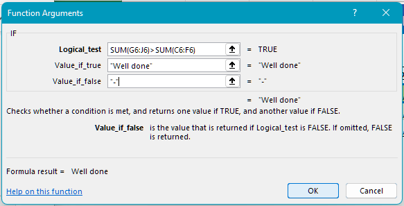
• Click OK.

Correct Formula Errors

Identify Different Error Types

Excel sometimes displays errors when using functions.

There are a few different errors with strange names, which make them easier to recognize. The main error values include #NAME?, #REF!, #VALUE!, #N/A and #DIV/0!

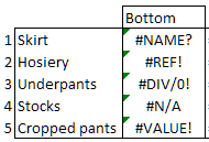
We can see how to correct these error types by displaying the five formulas used:

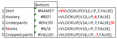
#NAME?

This error means that you have mistyped the VLOOKUP() function. In this case, there are two Vs.

• You simply need to correct the formula.

#REF!

This message indicates that the formula refers to a cell which cannot be found. In this example, the third argument of the function refers to column number 8, which is not included in the data range “J:P.”

• Check the cell references in your formula.

#DIV/0!

The error indicates that Excel is calculating a division by zero, which is impossible.

• Check the divisions in your formula, and look for zeros.

#N/A

Displays when your formula cannot find what it is looking for. This is a common error when using the VLOOKUP() function. In this case, the garment sought (“Stocks”) contains a syntax error, as there is a ’t’ in what should be “Socks.” Consequently, Excel cannot find this value.

• Check the data that your formula is looking for.

#VALUE!

This error can be more complicated, as it is a general error which is not linked to a specific problem. In this case, it is the third argument of the VLOOKUP() function, “-7,” which is causing the error. Excel is seeking a positive value rather than a negative value.

• Check each argument in your formula.

Find Error Cells

The first step is to find error cells and understand what has gone wrong.

Excel can help you with this. Simply use the icon in the “Formulas” tab.

• Select a worksheet which contains errors.

• Click on this button.

• Excel will help you to analyze the errors by finding them and providing an explanation.

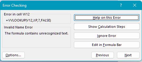
• Click Next to go to the next error.

Anticipate Errors

Sometimes, a formula might throw up an error which is entirely expected. For example:

• Potential zero value (sales, changes etc.)

• If the VLOOKUP() function cannot find a match

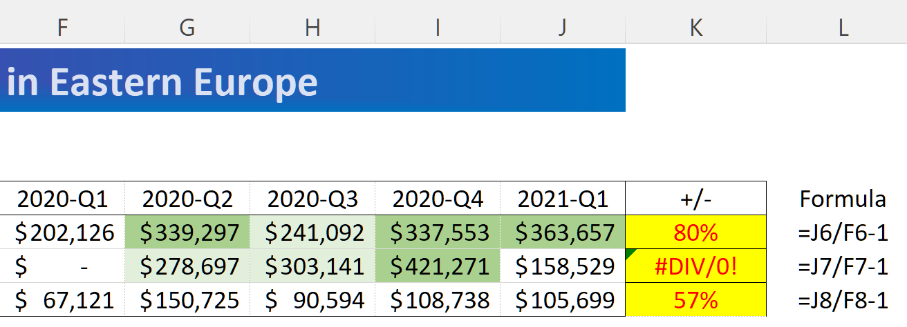
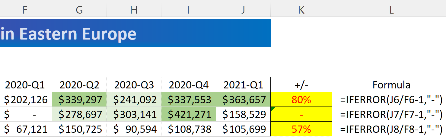
In this example, you want to calculate the change in sales between the first quarter of the current year and the first quarter of the previous year.

You need to allow for a quarter with no sales, which will bring up the error “#DIV/0!”

You’ll need to use the IFERROR() function to manage potential formula errors:

• The formula is: “If the change is an error, display a hyphen, otherwise display the change.”

• The basic syntax for the change formula is “J7/F7-1.”

• Display a hyphen in the case of an erroneous result: =IFERROR(J7/F7-1,“-”).

Over to You!

Download this file and do the following:

• Populate the “Opinion” column with the text “Great!” when the maximum sales for the last six quarters exceeds 5.2. Otherwise, display “-.” To do so, use the IF() formula with a nested MAX() formula, in the yellow cells.

• Collect the two error cells (cells with an orange background). The first displays 119%, and the second 139%.

• Modify the error cell (cell with a blue background) so that it displays a “-” when there is an error. Tip: use the IFERROR() function.

Answer Key

Look at the answer key and watch the video below to check your work.

Let’s Recap!

• You can nest a function inside another, if you replace an argument with a function. This allows you to tailor functions to your own requirements.

• Don’t forget to check the formulas in your file, and to correct any errors.

Your tables are now full of error-free formulas, and the cell formats adjust depending on the value. All you need to do now is work on the graphics! 😊