Consolidate Large Quantities of Data

Your boss has sent you a new data list, which includes the most recent sales. He asks you to add them to your recent analysis. To do so, you’ll need to consolidate all of the data.
What does consolidate mean?
Consolidating means grouping together different lists located on different tabs in a single, easy-to-use list.
Consolidate Several Data Ranges
Prepare Data Ranges for Consolidation
The new list is in exactly the same format as the original, unprocessed file that you received at the beginning of the training program (the full data list in part 2, chapter 3). You therefore process it in the same way, and transform it into a data table which is identical to the existing one.
Please download this file to follow the demonstration.
You end up with four identical tables for different periods:
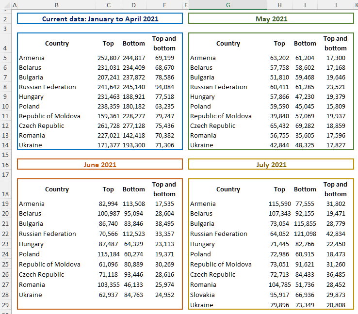
You notice that a new country (Slovakia) appears on the July data. You therefore have a table with an extra row.
Select Ranges for Consolidation
To consolidate this data:
Create a new worksheet, as this is where your consolidated data will go.
Go to the “Data” tab, “Data Tools,” and then click on the “Consolidate” icon.
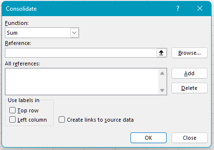
Leave the Function as “Sum,” as this is what you want to do.
In the Reference field, select the cell range from the first table, including the header row (B4:E15).
Click “Add” to add the selected range to the list.
Do the same for the other three tables.
Check the “Top row” and “Left column” boxes, as the source data has labels in these locations.
Also check “Create links to source data.”
Click OK.
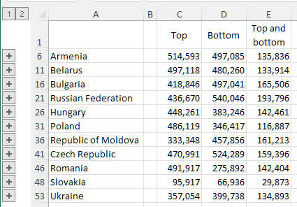
You’ll notice that the consolidated data includes grouped rows (little plus symbols on the left-hand side). These let you expand or collapse the detail of each source table.
Create a Pivot Table From Multiple Sources
Another way of consolidating different data sources is to use a Pivot Table. The advantage of this over the “Consolidate” tool is that you can mix complementary data.
Please download this file to follow the demonstration.
In this case, you’re going to combine two tables to cross sales data with country code data:
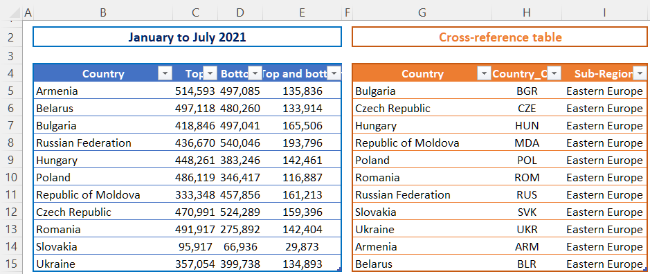
You’ll need to start by transforming your raw data into an Excel table (refer back to this chapter). Here, for the sake of clarity, they will be renamed as “Table1” and “Table2.”
Go to “Insert” and then “PivotTable.”
Type “Table1” in the source, and check the box “Add this data to the Data Model.”
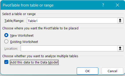
Click “OK.”
You’ll see that the fields display to the right of the screen, with a special icon next to “Table1.”
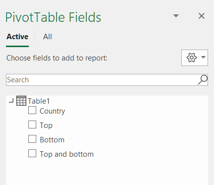
Check all of the boxes to populate the table.
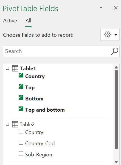
Click the “All” tab at the top of the box.
You’ll see that “Table2” is also displayed:
When you check a field under “Table2” to add it to your Pivot Table, you get the following message:
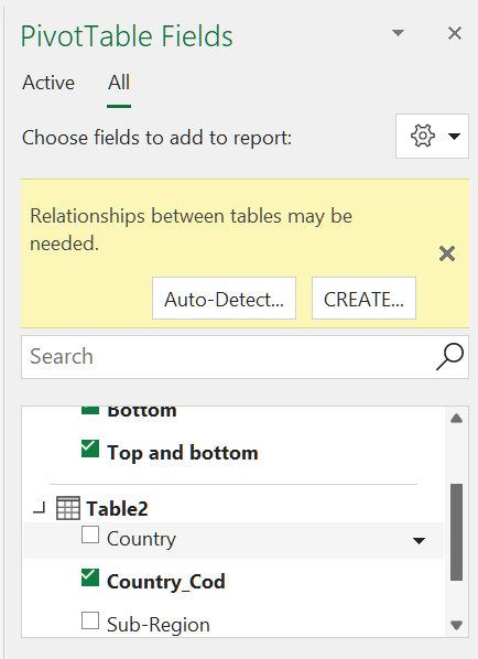
Click on “Create.”
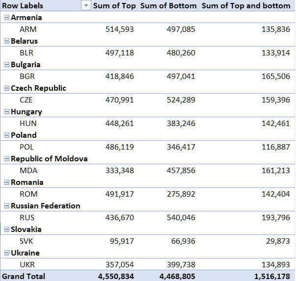
You’ll then need to tell Excel which fields the two tables share:
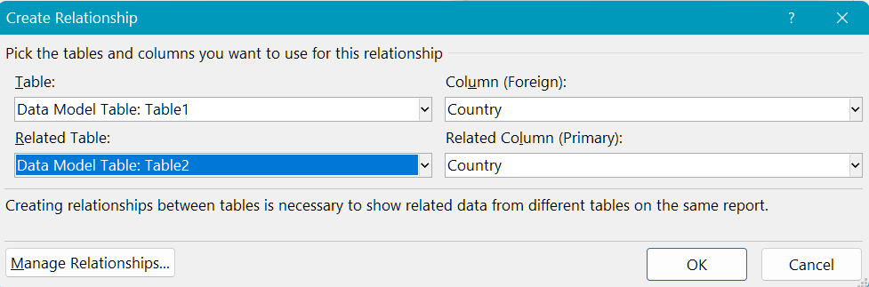
Ta-da! You have a Pivot Table which combines data from several different source tables! 😀
Over to You!
Download this file and do the following:
Use the “Consolidate” feature to consolidate data from the two worksheets “P4C2-Conso1” and “P4C2-Conso2” in a new worksheet.
In the “P4C2-TCD” worksheet, consolidate the two tables “My_Table1” and “My_Table2” in a single Pivot Table. The goal is to find total sales for pink blouses in Belgium.
Answer Key
You can find the answer key here and watch the video below to check your work.
Let’s Recap!
Consolidate multiple tables with the same layout using the “Consolidate” feature.
Cross-reference several tables with a shared field using Pivot Table data models.
You now know how to combine large quantities of data. 🥳 Join me in the next chapter to learn how to use this data more effectively!
