Enhance Your Table

Your data now looks something like this:

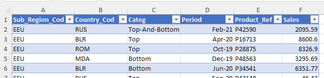
You can download this file if you need to.

Keep your original goal in mind. You need to use this data to answer two questions:

• How have Zarigual’s Western European sales been going since 2019, by garment and on a quarterly basis?

• Are the 2018 collection pants selling as well as the 2020 collection ones?

You notice that the region, country, and product names are not very clear. As it stands, you only have the codes (columns A, B, and E). You therefore ask your boss to send you a cross-reference table, so that you can complete your data list.

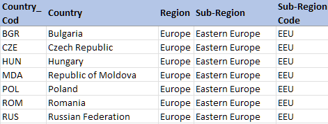
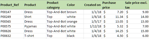
Your boss sends you two cross-reference tables (two tabs grouped together in a single workbook):

• One table for countries and regions

• And one table for products

Enhance Your Text and Number Data

Let’s start by adding the country and product names to your table. You can do this using the VLOOKUP() function.

The VLOOKUP() Function

This function allows you to add data from another Excel worksheet or workbook. Look carefully at the diagrams below to understand how it works. In this example, the data is in different workbooks:

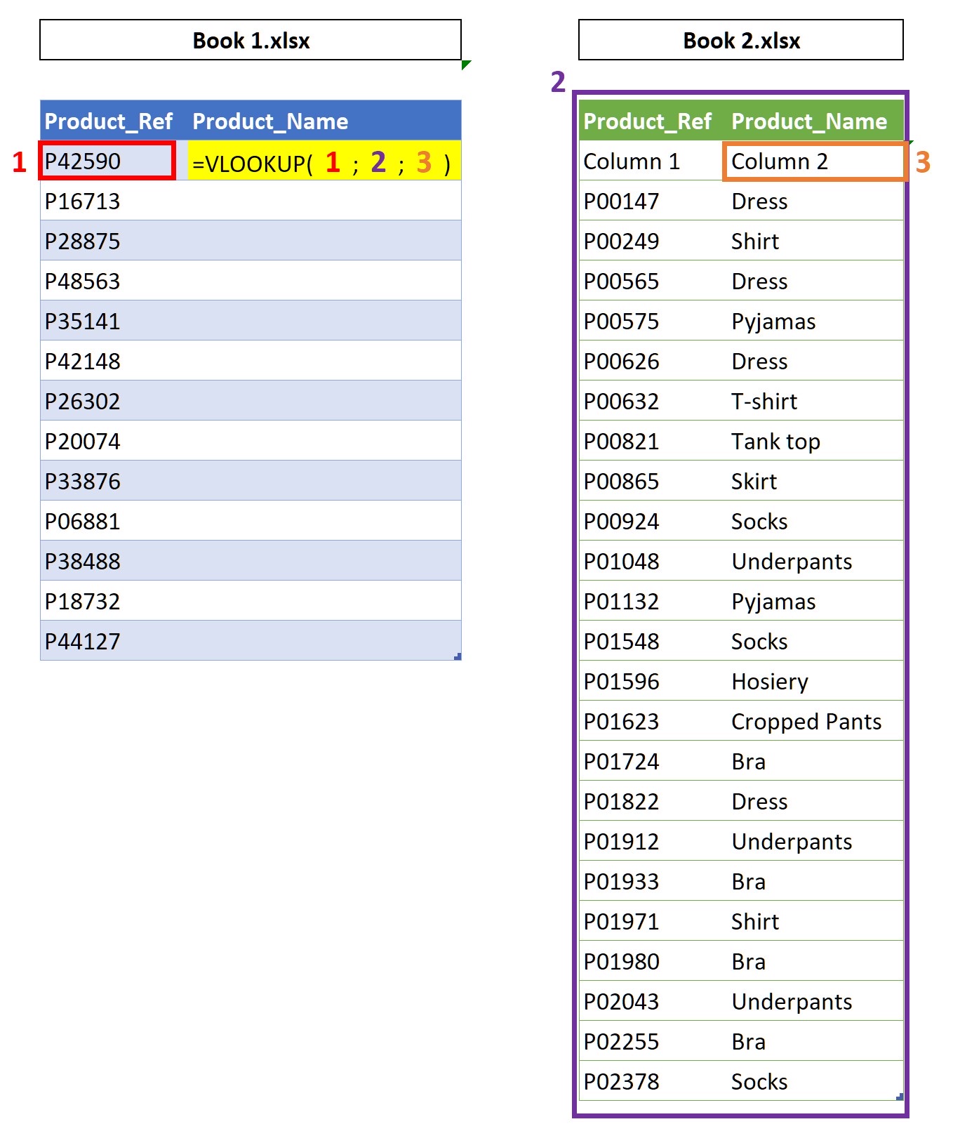
In this schema, you’ll see that the formula is broken down into four arguments, represented by the figures 1, 2, 3 and 4:

• Argument 1: the cell containing the data common to both files

• Argument 2: the cell range in which the new data is sought

• Argument 3: within the Argument 2 range, the number of the column containing the new data

• Argument 4: tells Excel if you would like to search for an approximate value (value TRUE), or an exact value (value FALSE).

In other words: “When searching for THIS DATA in column 1 of THIS RANGE, I will retrieve the information from THIS COLUMN by carrying out an EXACT MATCH search.”

• With the function syntax, it looks like this:

  • =VLOOKUP(THIS DATA, THIS RANGE, THIS COLUMN, EXACT MATCH) 

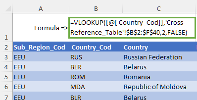
• The formula to find the country name therefore looks like this: =VLOOKUP(B2,Cross-reference_Table!$B$2:$F$40,2,FALSE).

Therefore, to add the country name to your table, you need to:

• add a new column to the right of the Country_Cod column.

• use the VLOOKUP() function to find the country code and country name match. 

You should get a result which looks like this:

You can then add all the product data from the product cross-reference table to your table!

Combine the INDEX() and MATCH() Functions

The VLOOKUP() function only works when the data common to the two databases is located in column 1 of the cross-reference table.

If this is not the case, you’ll need to use a combination of two functions, INDEX() and MATCH(). Both of these functions are straightforward to use, and are very powerful when combined! 😀

INDEX() helps you find the value of a cell within a data range. For example: “In THIS RANGE, what is the value of the cell in LINE 2 and COLUMN 1”?

MATCH() helps you find out the location of a specific value within a cell range. For example: “In THIS COLUMN, how many cells down will I find the EXACT VALUE “Bottom”?”

To use this combination:

• add two columns to the right of the region code “Sub_Region_Cod”:

  • The first one, named “MATCH”, contains the formula                                                =MATCH(A1,Cross-reference_Table!$F$1:$F$40,0).

  • The second one, named “INDEX”, contains the formula = INDEX(Cross-reference_Table!$E$1:$E$40,B3).

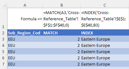
So now you can see how two straightforward functions work really well as a team! 😊

Enhance Your Date Data

Your data contains monthly sales, and in order to answer the first question that your boss has asked you, you need to create quarterly data.

There are many different Date functions in Excel, but unfortunately none of them can create the number of the quarter directly from a date. 😕 Don’t worry, there are alternatives! This is a two-step process:

Create a Quarter Column

As a quarter covers three months, you can use the month number to work out the quarter:

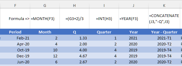
• Insert five columns to the right of the “Period” field.

• Column 1, named “Month,” finds the sales month (from 1 to 12) using the MONTH() function:

  • The G1 formula is =MONTH(F1).

• Column 2, named “Q,” divides the month number by three. The goal is to obtain a value of 1 or more for the first three months, 2 or more for the next three months, and so on:

  • The formula is =(G1+2)/3.

• Column 3, named “Quarter,” contains a non-decimalized figure of between 1 and 4, based on the value of the previous column, using the INT() function:

  • The formula is =INT(H1).

• Column 4, named “Year,” extracts the year from the “Period” field using the YEAR() function:

  • The formula is =YEAR(F1).

• Column 5, named “Year-Quarter,” combines the year and the quarter to create a field that Excel can use:

  • The formula is =CONCATENATE(J1,“-T”,I1).

The Year-Quarter field now works and can be used! 😊

Calculate the Interval Between the Product Creation Date and its Sale Date

Excel offers two solutions to calculate the interval between two dates:

• Calculate a time period in calendar days using the DAYS() function

• Calculate a time period in working days, i.e., excluding weekends (with the option to include public holidays), using the NETWORKDAYS() function

There are two very similar Excel functions called DAY() and DAYS(). Make sure you don’t mix them up! 😅

• The DAY() function replicates the day number of a date (number from 1 to 31).

• The DAYS() function calculates the interval between two dates.

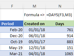
In this case, you’ll need to use the DAYS() function, as Zarigual’s stores are open seven days a week:

• Insert a “Created on” column to the right of the Product column.

• Use the formula =DAYS(F1,M1).

So now you know how to calculate a time period in calendar days or in working days! 😊

Over to You!

Your data table is nearly done! You just need to add some data to it so you can answer the two questions from your boss.

Using this downloadable file:

• Using the VLOOKUP() function, add the “Country” column from the “Cross-reference_Table” tab to the “P2C5-Over_to_you” tab.

• Using the INDEX() and MATCH() functions, add columns H to N (green columns) from the “Cross-reference_Table” tab to the “P2C5-Over_to_you” tab.  

• Add an “Interval in working days” column to calculate the interval between the “Created on” date and the “Period” date, with public holidays not included in the formula.

Answer Key

You can find the answer key here and watch the video below to check your work.

Let’s Recap!

• You can add data from other worksheets or files to your table, using the VLOOKUP(), INDEX() and MATCH() functions.

• You can calculate intervals between two dates using the DAYS() and NETWORKDAYS() functions.

Well done! Your table is now operational! In the second part of this course, you will complete the next step of creating a dashboard. But first, test your knowledge with a quiz!