Highlight information automatically with conditional formatting
Conditional formatting is a great way to call attention to the values in your spreadsheet. There are a lot of options when you conditionally format data. We'll end this part of the course with a short chapter about this!
Decide what you want to call attention to
The first step in conditional formatting data is to think about what values you want to call attention to. This step is the most important because it will be the basis for the rules you set.
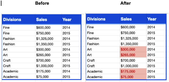
In the example below, let’s say I want to call attention to any values less than $500,000 because we want to highlight poor figures.
Without conditional formatting, I have to spend more time reading all of the cells in the second column and figuring out which values are less than $500,000.
See how the data jumps off the page?
Set up conditional formatting
To conditionally format your data, navigate to Format on the menu bar, then select Conditional Formatting.
Select the cells to format
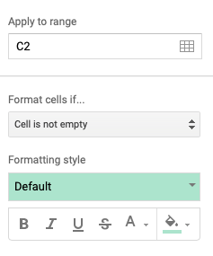
If not already done, select or identify either one cell or a range of cells you want to format, based on the values in the Apply to range section.
Conditional formatting dialog box
Set up the condition
Click on the Format cells if… dropdown arrow to see the conditions on which to format your data. Common conditions include mathematical functions like less than or greater than as well as time-based conditions.
Set the formatting style
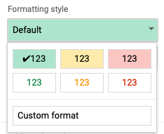
Once the condition is set, then the formatting style can also be set. There are some preset options as well as a custom format.
Conditional formatting styles
In Google Sheets, you can add rules to help refine your conditions and even apply a color gradient to the data!
Your Turn!
You are sent a spreadsheet with sales data and need to highlight the best and worst sales by division in recent years.
You decide to highlight good news in green and bad news in red.
Using the data in this spreadsheet, conditionally format the data to highlight sales less than or equal to $500,000, and greater than or equal to $1,000,000.
You decide to try out your formatting skills and edit the color of the values as well.
Shade the background of cells with sales less than or equal to $500,000 in bright red with the value in white.
Shade the background of cells with sales greater than or equal to $1,000,000 in light green with the value in dark green.
Check your Work!
Now check that you managed to set a proper conditional formatting by changing the values in the cells and verify that it changes the color as expected. You can find an example by downloading this file.
Let’s recap!
The purpose of conditional formatting data is to draw attention to it.
Data highlighted in green is seen as positive, while red is viewed as negative.
There are three steps to setting up conditional formatting:
Select the cell(s) you want to apply the condition to.
Identify the condition (or create your own).
Select the formatting to highlight the values that meet your condition(s).
Well done, you made it to the end of Part 2! Let’s check what you learned in Part 2 of this course in a quiz before we move on to analyzing data.