Train a Supervised Machine Learning Model

Feature Engineering

Feature engineering is the creation of new input or target features from existing features. The objective is to create ones that do a better job of representing a machine learning problem to the model. By doing so, you can improve the accuracy of the model.

Good feature engineering can be the difference between a poor model and a fantastic one! More often than not, you will find that you can squeeze more out of your models through careful feature selection than any amount of algorithm tuning.

For example, consider the following dataset showing property prices:

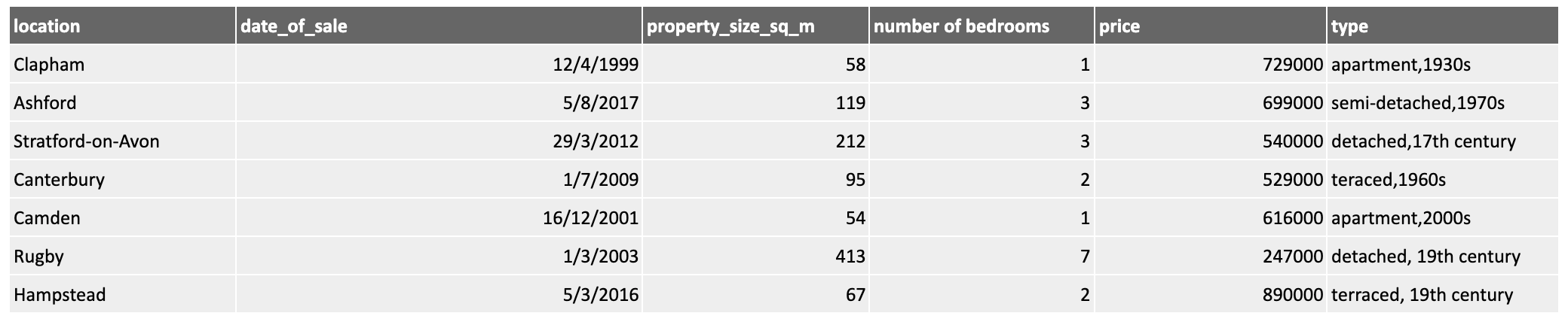
While the data is clean, any machine learning activity would benefit from some additional processing of the data, perhaps presenting it to a machine learning tool in this form:

Here you can see, in yellow, some new features derived from the existing ones. We have added the district to make inferences at the district level. The date was broken down into year and month components to look for patterns across time as well as seasonal ones. We have derived metrics such as the price_per_square_metre and price_per_bedroom and split the two parts of the property type into separate columns. All of these offer additional options to choose from when selecting features later.

By spending time performing feature engineering, you can focus on the important, high-quality features, rather than throwing raw data at a model and hoping for the best!

Feature engineering is not a mechanical, linear process. You need to adapt your techniques in response to the data you see, the problem you are trying to solve, and your domain knowledge. You may also want to consult others to utilize their domain knowledge.

You may also decide you need more, different, or better data and spend some time sourcing supporting data.

And once you've built your model, you may come back to do more feature engineering to see if you can improve the performance.

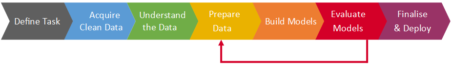
This illustrates the iterative nature of building machine learning models.  As we have discussed before, the process is not linear, and you may go back at any point to improve a previous activity:

In this chapter, we will look at some of the techniques you can use to engineer features from data. This is not an exhaustive list, but it includes the most common techniques you will need. The data and code used for each section are on the GitHub repository for this course.  There is a short screencast at the end of each section that demonstrates the technique.

Binning

Binning, (also called banding or discretisation), can be used to create new categorical features that group individuals based on the value ranges of existing features.  

You can use binning to create new target features you want to predict or new input features.

Numerical Binning

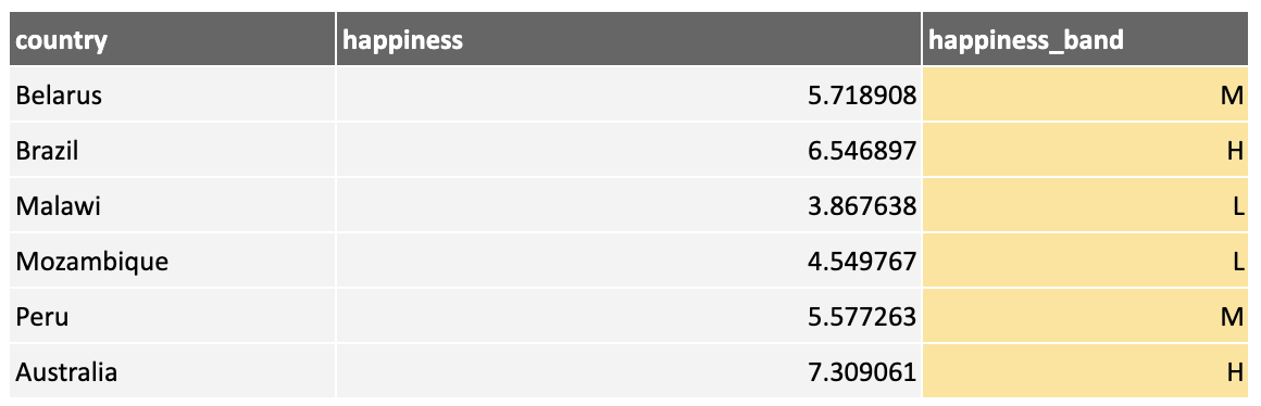
For example, using data from the World Happiness Report, we create a new feature, happiness_band, by binning the happiness feature into low, medium, and high bands:

Numerical Binning With Python

Let's look at how to perform binning in Python. First, load in a dataset containing country names and their happiness scores:

df1 = pd.read_csv("fe_binning.csv")
df1.head()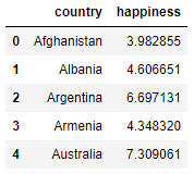

Bin the data into low, medium, and high bands using the following code:

# Allocate happiness to bins
binned = pd.cut(df1["happiness"], bins = [0,4.5,6,10], labels = ["L","M","H"])

# Add the binned values as a new categorical feature
df1["happiness_band"] = binned

The  bins  parameter defines the boundaries of the bins. In this case, I have chosen to split the data into bins containing countries with happiness values of 0 to 4.5, 4.5 to 6, and 6 to 10.

The  labels  parameter allows you to name each bin.   Note there is one less label than bin boundary (because we need four boundaries to make three bins).

Here's the new feature:

df1.head()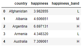

Inspect the number of individuals in each of the created classes:

df1.groupby("happiness_band").size()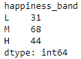

Categorical Binning

The above is an example of binning on numerical features.  You can also apply binning to categorical features.  Here are the countries binned into their global region:

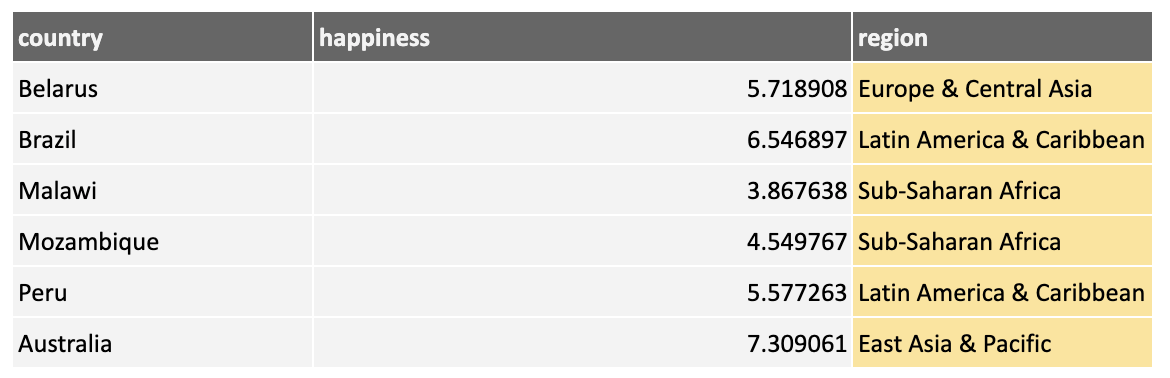
Grouping countries into broader regions could help in our model creation as a country's region has strong powers for predicting our target feature.

Categorical Binning With Python

Let's see how the above can be carried out in Python.

We'll load a mapping table, mapping countries to their region:

mapping = pd.read_csv("country_region.csv")

And join the country on the original data to the region using the mapping table.

df1 = pd.merge(df1, mapping, left_on='country', right_on='country', how="left")

Use left as the  how  parameter to specify that all rows in the left table (df1) are included and joined to any matching rows in the right table (mapping).  Any rows in df1 that have no match in mapping will receive a null value for the region.

Note that there are other ways you can perform this mapping (e.g., using a dictionary and the pandas map function). Your coding approach will vary according to the task in hand!

Splitting

Splitting can be used to split up an existing feature into multiple new features.

Date/Time Decomposition

A common use of splitting is breaking dates and times into their component parts.

Consider the following data, showing domestic fire calls to the London Fire Department over a period a time:

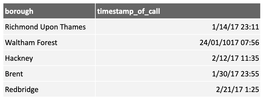
The date column could be used for analysis, but it has very little information value. However, if we split it into the year, month, day, and day of the week, we can derive models that, for example, explore whether fires in London tend to occur on particular days of the week, thus using our domain knowledge.

Date/Time Decomposition With Python

Let's look at date splitting in Python.  First, let's load some data and examine the first few rows:

df2 = pd.read_csv("fe_splitting.csv")
df2.head()

Use the  to_datetime()  function to convert the object to a date/time type:

df2["timestamp_of_call"] = pd.to_datetime(df2["timestamp_of_call"])

Checking again, you can see the timestamp_of_call feature is now a date:

df2.dtypes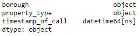

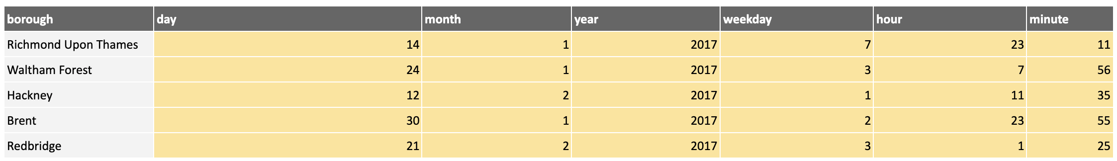
Now add some new features by extracting the components of the timestamp_of_call:

df2["day"] = df2["timestamp_of_call"].dt.day
df2["month"] = df2["timestamp_of_call"].dt.month
df2["year"] = df2["timestamp_of_call"].dt.year
df2["weekday"] = df2["timestamp_of_call"].dt.weekday
df2["hour"] = df2["timestamp_of_call"].dt.hour

And you can see that we now have new features:

df2.head()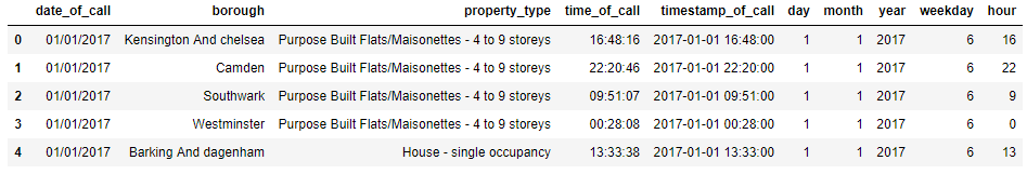

Check that everything has converted by looking at the non-null counts in each column match:

df2.isnull().mean()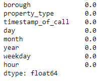

Compound String Splitting

Sometimes data comes with compound strings, which are strings made up of multiple items of information. One example is in the London Fire Department data. The property_type contains information about the property type (e.g., Purpose Built Flats/Maisonette) and the size (e.g., 4 to 9 stories).

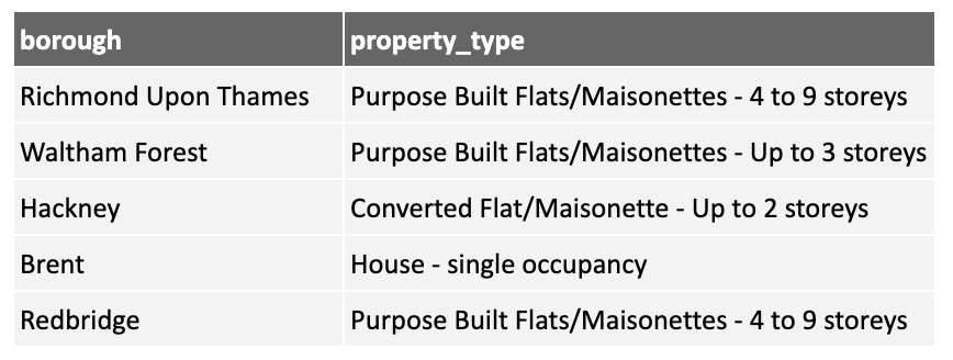
Having these two pieces of information combined does not help our model!  So we can split it into two separate features:

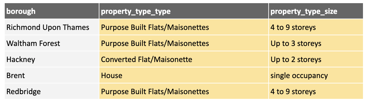
Splitting Compound Strings With Python

Let's reload the London Fire Department data and look at string splitting in Python:

df3 = pd.read_csv("fe_splitting.csv")
df3.head()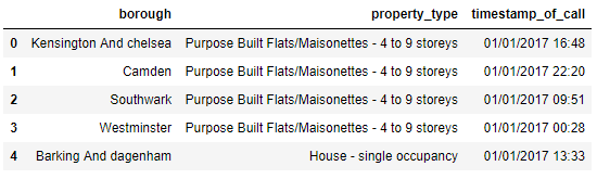

The first thought may be to split the data at the hyphen. However, some rows may not contain one, while others may have multiples. This could cause a problem. Let's check the data to see the unique values for property_type we need to deal with:

df3["property_type"].unique()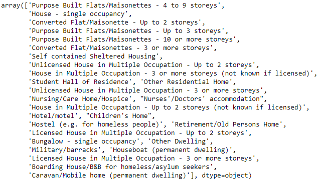

Looking at these individually, there are no multiple hyphens, but there are some that don't have any, which will create null entries when split. We will need to deal with these later if we want to use this new feature for machine learning.

Let's do the split, and confirm the results:

df3[['property_type_type', 'property_type_size']] = df3["property_type"].str.split("-",expand=True)
df3.head()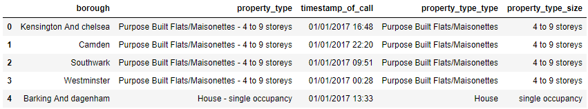

A quick check confirms that the property_type_size column contains nulls as there was no hyphen to split on:

df3.isnull().mean()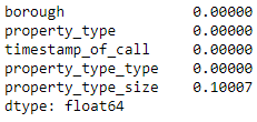

You would need to make an informed decision about what to do about these nulls, as explained in the data cleansing section of the course!

One-Hot Encoding

The sklearn libraries can't build models with categorical data, so if you want to build models using categorical features, you need to convert them to numerical ones. One-hot encoding is a way of doing this.

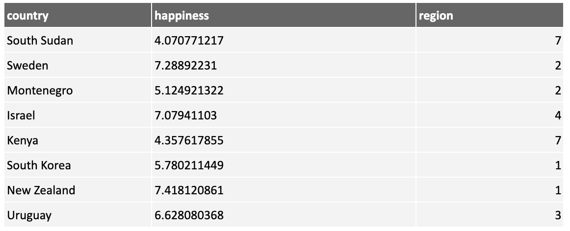
Consider the following table of countries from the happiness dataset:

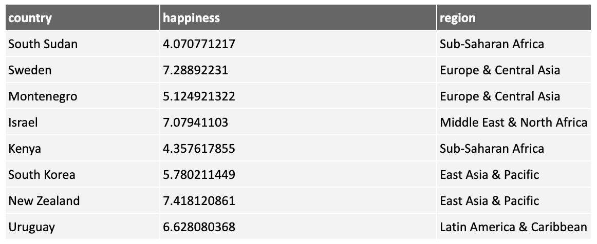
The region column is categorical, so to enable sklearn to use it, convert it to numerical.

You could use a lookup table to map these regions to numbers:

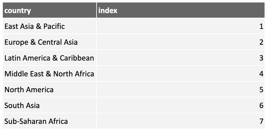
Then the data will look like this:

This approach introduces a problem. Each region has been assigned a value. While the size is meaningless (it's just an id), most machine learning algorithms will infer some meaning, such as South Asia is "greater than" East Asia & Pacific. This will lead to meaningless models, so the approach is not useful.

One-hot encoding places each category in a column as a new feature, with a 1 or 0 to indicate if it's on or off. Here is the result of applying one-hot encoding to the above dataset: 

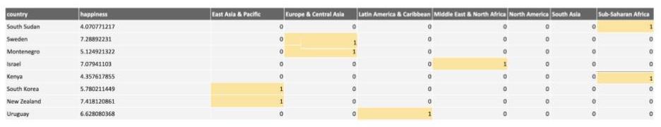
These new categories are called dummy variables.

One-Hot Encoding With Python

Now let's see how to perform one-hot encoding with Python. First, let's load the data:

df4 = pd.read_csv("fe_one_hot.csv")
df4.head()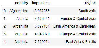

Use the pandas  get_dummies()  function to convert the required column to dummy variables:

region_one_hot = pd.get_dummies(df4.region)
region_one_hot.head()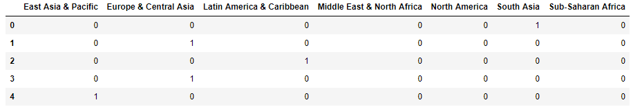

Join the new columns back onto the dataset, dropping the region column that we just encoded:

df4 = df4.join(region_one_hot).drop('region', axis=1)
df4.head()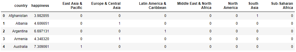

Calculated Features

In some cases, you can create new features using calculations based on existing features.

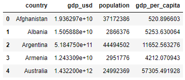
For example, consider the following data showing the total GDP and population by country:

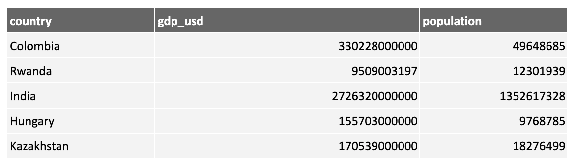
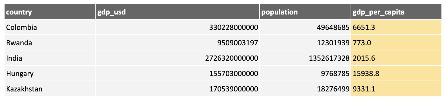
Both the GDP and population tend to be larger for larger countries and can lead to models too influenced by size. Dividing GDP by population results in a new measure, gdp_per_capita, which could be more useful:

You could perform various calculations, generating ratios such as GDP per capita, differences between two values, or even more complex calculations. You could also create aggregations by grouping data, then summing, taking the mean, using min or max, and so on.

The nature of the calculations depends on having appropriate domain knowledge.

Calculated Features in Python

Let's load some data:

df5 = pd.read_csv("fe_calculated.csv")
df5.head()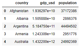

We can easily perform a calculation on existing features to create a new feature:

Recap

Feature engineering is an important step! It allows you to create new features that can boost a model's chances of success. Utilize your domain knowledge when engineering features and bring in supporting data where helpful

Remember: Machine learning is an iterative process, so once you have built your model, return to feature engineering to see if you can make any improvements.

We looked at a few techniques:

• Binning

  • Numerical binning

  • Categorical binning

• Splitting

  • Date/time decomposition

  • Compound string splitting

• One-hot encoding to deal with categorical features

• Calculated features

In the next part, we will build a classification model. But for now, it's time to test your knowledge!