Train a Supervised Machine Learning Model

Now that you understand how the decision trees and logistic regression algorithms work, let's put them into action by building some classification models in Python. We are going to follow the same process we used in Part 1, but with a slightly more realistic example.

• The dataset is a little larger, both in terms of the number of sample points and features.

• The data is a little messy, so some cleanup will be necessary.

• We will need a little feature engineering along the way.

• We have two available algorithms, so we need to decide which to use.

A Quick Refresher

Here is a quick reminder of the code written in Part 1 to build a model to predict happiness. Refer back to that chapter if you need a refresher.

# Import Python libraries for data manipulation and visualisation
import pandas as pd
import numpy as np
import matplotlib.pyplot as pyplot

# Import the Python machine learning libraries we need
from sklearn.model_selection import train_test_split
from sklearn.tree import DecisionTreeClassifier
from sklearn.metrics import accuracy_score

# Import some convenient functions.  This can be found on the course github
from functions import *

# Load the data
dataset = pd.read_csv("world_data_really_tiny.csv")

# Inspect first few rows
dataset.head(12)

# Inspect data shape
dataset.shape

# Inspect descriptive stats
dataset.describe()

# View univariate histgram plots
histPlotAll(dataset)

# View univariate box plots
boxPlotAll(dataset)

# View class split
classComparePlot(dataset[["happiness","lifeexp","unemployment"]], 'happiness', plotType='hist')

# Split into input and output features
y = dataset["happiness"]
X = dataset[["lifeexp","unemployment"]]

# Split into test and training sets
test_size = 0.33
seed = 7
X_train, X_test, y_train, y_test =  train_test_split(X, y, test_size=test_size, random_state=seed)

# Select algorithm
model = DecisionTreeClassifier()

# Fit model to the data
model.fit(X_train, y_train)

# Check model performance on training data
predictions = model.predict(X_train)
print(accuracy_score(y_train, predictions))

# Evaluate the model on the test data
predictions = model.predict(X_test)
print(accuracy_score(y_test, predictions))

Our Dataset

This chapter will use datasets from the World Bank, Gapminder, and the World Happiness Report.

For this course, I've selected a few of the features available from these sources, cleaned and performed imputation of the data to provide the most recent measures for each country up to 2015.

When doing any machine learning task, it is important to understand as much about the meaning of the data as possible. Here are the descriptions of the columns from the respective sources:

• Country: Country name.

• Happiness: The national average response to the question: “Please imagine a ladder, with steps numbered from 0 at the bottom to 10 at the top. The top of the ladder represents the best possible life for you and the bottom of the ladder represents the worst possible life for you. On which step of the ladder would you say you personally feel you stand at this time?”

• Income: Gross domestic product per person adjusted for differences in purchasing power (in international dollars, fixed 2011 prices, PPP based on 2011 ICP).

• Lifeexp: The average number of years a newborn child would live if current mortality patterns were to stay the same.

• Sanitation: The percentage of people using at least basic sanitation services, that is, improved sanitation facilities that are not shared with other households. 

• Water: The percentage of people with at least basic water services. 

• Urbanpopulation: Urban population refers to people living in urban areas as defined by national statistical offices. 

• Unemployment: Percentage of total population that has been registered as long-term unemployed during the given year.

• Literacy: Adult literacy rate is the percentage of people ages 15 and above who can clearly read and write a short, simple statement on their everyday life.

• Inequality: Gini income inequality in a society. A higher number means more inequality.

• Murder: Mortality due to interpersonal violence, per 100,000 standard population, age adjusted. This rate is calculated as if all countries had the same age composition of the population.

• Energy: Energy use refers to use of primary energy before transformation to other end-use fuels, which is equal to indigenous production plus imports and stock changes, minus exports and fuels supplied to ships and aircraft engaged in international transport.

• Childmortality: Death of children under five years of age per 1,000 live births.

• Fertility: Total fertility rate. The number of children that would be born to each woman with prevailing age-specific fertility rates.

• HIV: The total number of persons of all ages estimated to be infected by HIV, including those without symptoms, those sick from AIDS, and those healthy due to treatment of the HIV infection.

• Foodsupply: Calories measures the energy content of the food. The required intake varies, but it is normally in the range of 1500-3000 kilocalories per day. One banana contains approximately 100 kilocalories.

• Populationtotal: Total population.

Let's build a model!  You can find the code on the course GitHub repository.

Part 1:

Watch this screencast showing the first stages: defining the task and acquiring and cleaning the data.  Then read the notes below.

Import the Libraries

Let's start by importing the necessary libraries - pandas, NumPy, and matplotlib; some functionality from sklearn; and a small library of convenience functions used specifically for this course. Feel free to open up functions.py to see what's inside it.

# Core libraries
import pandas as pd
import numpy as np
import matplotlib.pyplot as pyplot

# Sklearn processing
from sklearn.preprocessing import MinMaxScaler
from sklearn.model_selection import train_test_split

# Sklearn classification algorithms
from sklearn.tree import DecisionTreeClassifier
from sklearn.linear_model import LogisticRegression

# Sklearn classification model evaluation function
from sklearn.metrics import accuracy_score

# Convenience functions.  This can be found on the course github
from functions import *

The Process

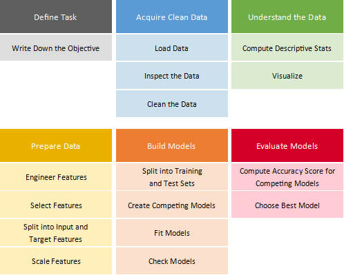
Here's a reminder of the process from Part 1 of the course that we'll be using.

Define the Task

The task is to:

Make predictions about a country's life expectancy (L/M/H bands) from a set of metrics for the country.

Acquire Clean Data

Load Data

Load the dataset.

dataset = pd.read_csv("world_data.csv")

Inspect Data

Identify the number of features (columns) and samples (rows):

dataset.shape

 (194, 17)

Take a quick look at the data to understand what you are dealing with:

dataset.head()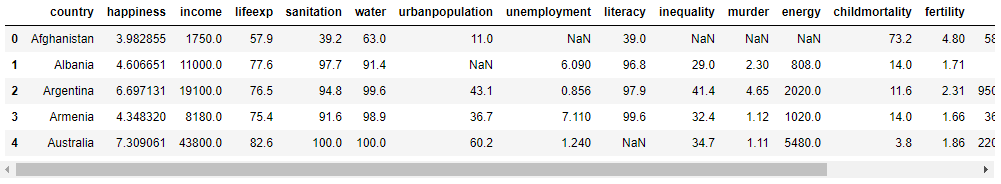

Check that there are sensible data types for each feature. For example, we don't want any numeric features to show up as an object type.

dataset.dtypes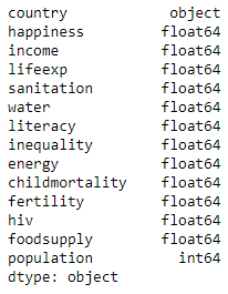

Check if there are nulls:

dataset.isnull().mean().sort_values()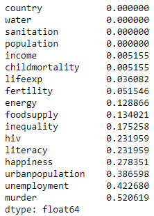

Clean Data

The numbers represent the percentage of null rows in each feature. Some of these features (murder, urbanpopulation, unemployment) are sparsely populated. If we were to impute the nulls, we would be estimating a large number of values. I am going to discard them for now but may come back to them again later (remember, this is an iterative process).

dataset = dataset.drop(["murder","urbanpopulation","unemployment"], axis=1)

For the others, I will just impute with the mean value of the feature.  Again, I may want to come back to this later.

# Compute the mean for each feature
means = dataset.mean().to_dict()

# Impute each null with the mean of that feature
for m in means:
    dataset[m] = dataset[m].fillna(value=means[m])

Confirm there are no nulls:

dataset.isnull().mean()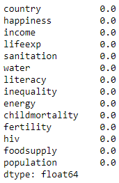

Part 2:

Watch this screencast showing the next stages: understanding the data.  Then read the notes below.

Understand the Data

Compute Descriptive Stats

Let's calculate some descriptive stats. These give you an idea of the range and spread of values for each feature. It also gives you a chance to check for anything unexpected, such as statistics that don't match the description of the feature. This may indicate erroneous data, either from the source or the cleanup process.

dataset.describe()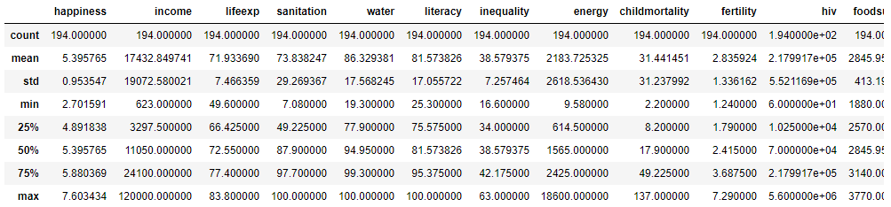

Visualize

A correlation matrix can be used to spot correlations between the features. We hope to see some good correlations of lifeexp with other features, as that's the one we want to predict. Let's use one of the convenience functions from  functions.py:

correlationMatrix(dataset)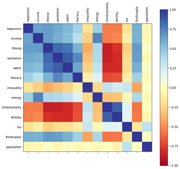

The color bar on the right shows the colors representing different levels of correlation.

Look at the lifeexp column. You can see that sanitation, water, foodsupply, and happiness are in dark blue, indicating strong positive correlations with lifeexp. Childmortality and fertility are in dark red, indicating strong negative correlations with lifeexp. Do these observations fit with your understanding of factors that may influence life expectancy? If they do, that's good news as you can expect the model to pick this up and model your real-world understanding! This demonstrates the use of domain knowledge to the task in hand!

You can also plot some box plots to understand the distribution of each feature. Again, do they reflect your understanding of the data? Are there any surprises? If there are, investigate them further!

boxPlotAll(dataset)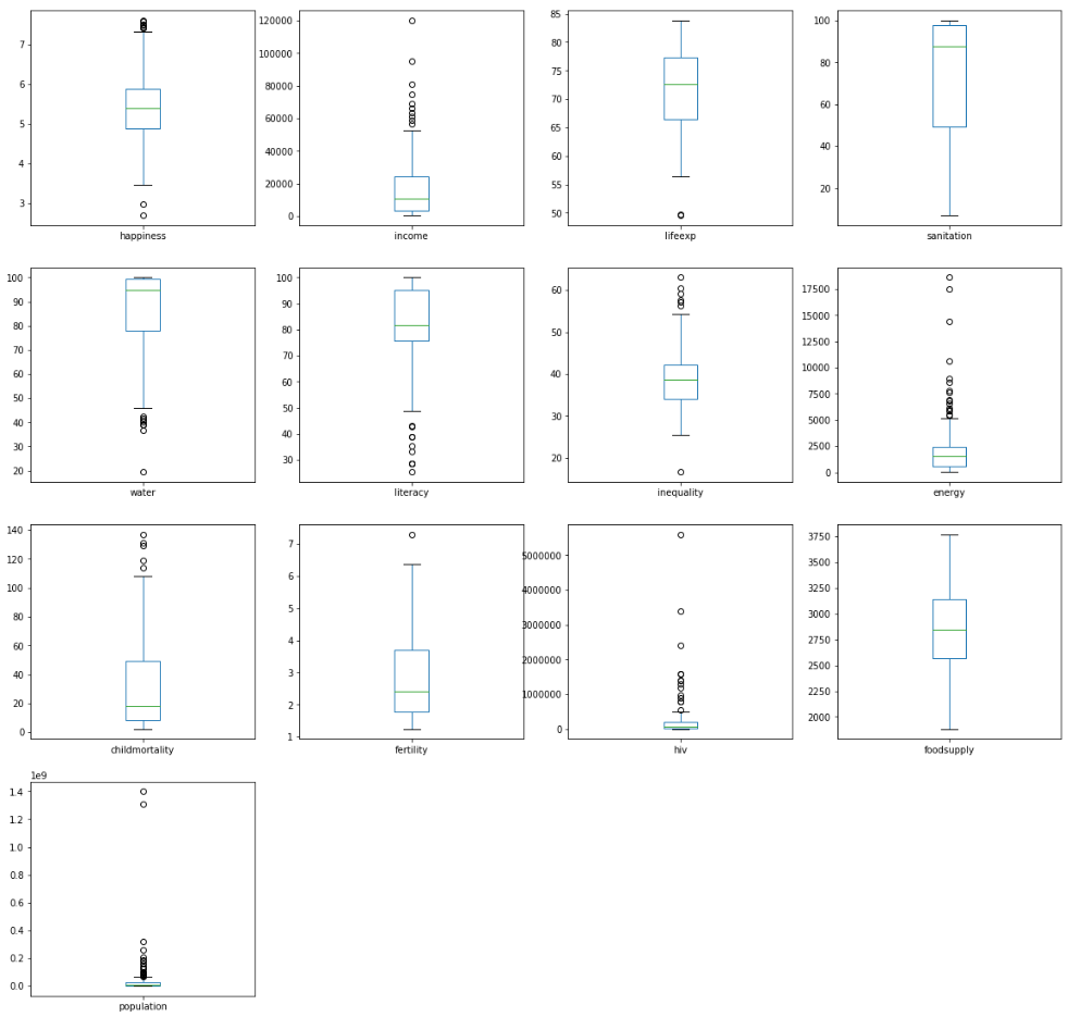

Part 3:

Watch this screencast showing the next stage: preparing the data.  Then read the notes below.

Prepare Data

Feature Engineering

The task was defined as:

Make predictions about a country's life expectancy (L/M/H bands) from a set of metrics for the country.

However, lifeexp is currently a continuous numeric feature. The data should be binned into L, M, and H bands. You learned about this technique in the chapter on feature engineering. So, let's add the new binned feature. The  appendEqualCountsClass() function can be found in functions.py.

dataset = appendEqualCountsClass(dataset, "lifeexp_band", "lifeexp", 3, ["L","M","H"])

Let's see if the results were what we expected: three bands with the same number of sample points in each:

dataset.lifeexp_band.value_counts()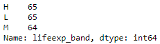

And let's check a few rows, to confirm it has worked as expected:

dataset[['lifeexp','lifeexp_band']].head()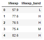

Select Features and Split Into Input and Target Features

Now we need to decide which columns to use as input features and which is our target feature. Let's select lifeexp_band as our target feature (the one we will predict) and everything else as the input features (the ones we will use to make the prediction).

y = dataset["lifeexp_band"]
X = dataset[['happiness', 'income', 'sanitation', 'water', 'literacy', 'inequality', 'energy', 'childmortality', 'fertility', 'hiv', 'foodsupply', 'population']]

Scale Features

When we ran dataset.describe() above, you saw that the range of values between the min and max was different for different features. Sanitation ranged from 7 to 100, but income ranged from 623 to 120,000. Many algorithms will not perform optimally with data on such vastly different scales. To prevent this, scale the data before building the model. There are a few approaches. In this case, I will use the  MinMaxScaler(), which scales the data so every feature ranges from 0 to 1.

# Rescale the data
scaler = MinMaxScaler(feature_range=(0,1))
rescaledX = scaler.fit_transform(X)

# Convert X back to a Pandas DataFrame, for convenience
X = pd.DataFrame(rescaledX, columns=X.columns)

Look at what this scaling has done. Every feature now has a min of 0 and a max of 1:

 X.describe()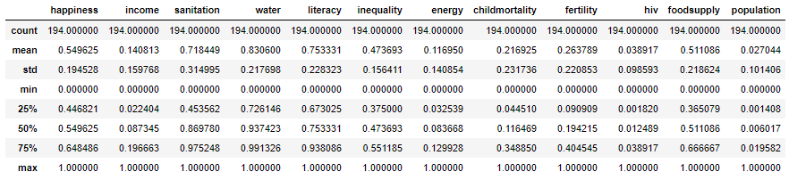

Part 4:

Watch this screencast showing the next stages: building and evaluating the models.  Then read the notes below.

Build Models

In the previous chapters, you learned about two algorithms for performing classification tasks: decision trees and logistic regression. It's great to have a choice, but with choice comes a little anxiety - which one should you choose?! Fear not! There is a simple way to decide: build two models and see which one performs the best!

Split Into Test and Training Sets

We want both models to have a fair opportunity to triumph! So we need to present both with identical training and test sets. We will generate them once, using a specific seed, so we can get the same random sample each time we run this code.

test_size = 0.33
seed = 1
X_train, X_test, Y_train, Y_test = train_test_split(X, y, test_size=test_size, random_state=seed)

Create Multiple Models, Fit and Check Them

Let's build both models and fit with the training data.  First, the decision tree model:

# Build a decision tree model
model_dt = DecisionTreeClassifier()
model_dt.fit(X_train, Y_train)

Then the logistic regression model:

# Build a logistic regression model
model_lr = LogisticRegression(solver='lbfgs', multi_class='auto')
model_lr.fit(X_train, Y_train)

We now have two trained models.

Check the Models

At this stage, we can check how well the models performed on the training data itself, and compute the accuracy score for each model. The accuracy score is:

$\$\backslash (accuracy\; score\; =\; \backslash frac\{number\; of\; correct\; predictions\}\{total\; number\; of\; predictions\}\backslash )\$$

Let's compute the accuracy score for each of model based on the training data:

# Check the model performance with the training data
predictions_dt = model_dt.predict(X_train)
print("DecisionTreeClassifier", accuracy_score(Y_train, predictions_dt))

DecisionTreeClassifier 1.0

# Check the model performance with the training data
predictions_lr = model_lr.predict(X_train)
print("LogisticRegression", accuracy_score(Y_train, predictions_lr))

LogisticRegression 0.8217054263565892

The accuracy score for each model predictions with the training data is below each code block. Based on the training data, the decision tree has done a great job, getting 100% of the classifications right! However, we can't rely on testing with our training data (remember, we are data scientists). So, we need to evaluate the model using the test data.

Evaluate Models

Now to evaluate the models by testing with the test set:

predictions_dt = model_dt.predict(X_test)
print("DecisionTreeClassifier", accuracy_score(Y_test, predictions_dt))

DecisionTreeClassifier 0.6461538461538462

predictions_lr = model_lr.predict(X_test)
print("LogisticRegression", accuracy_score(Y_test, predictions_lr))

LogisticRegression 0.7230769230769231

The tables have turned!  Logistic regression shows a better accuracy score on the test data, despite the fact that the decision tree performed better on the test data.

Now to declare the winner - logistic regression!

model = model_lr

Summary

Here's a summary of the process and the specific steps we performed to complete this particular machine learning task.

Iterate!

I've mentioned this word a few times in this course: iterate! I keep mentioning it because it's important and sometimes doesn't come across in beginner courses on machine learning. Although we sometimes describe machine learning processes as linear:

At this stage, you want to improve the accuracy of the created model. You may want to go back and do some more feature engineering:

Or revisit cleanup:

Or try some different algorithms or tune the algorithms:

Part 5:

Watch this screencast showing the inspection of the models.  Then read the notes below.

Inspect the Models

For a better understanding, you can look inside the models. Decision trees and logistic regression use very different ways of building models, so when you look under the hood, you see quite different things!

Decision Tree

You've seen a simple decision tree. Here is the one created for this exercise.  The text is a bit small to read, but just admire its complexity for a moment!

To run this code, you need to install  graphviz  as described in Part 1.  The  viewDecisionTree()  function can be found in  functions.py.

viewDecisionTree(model_dt, X.columns)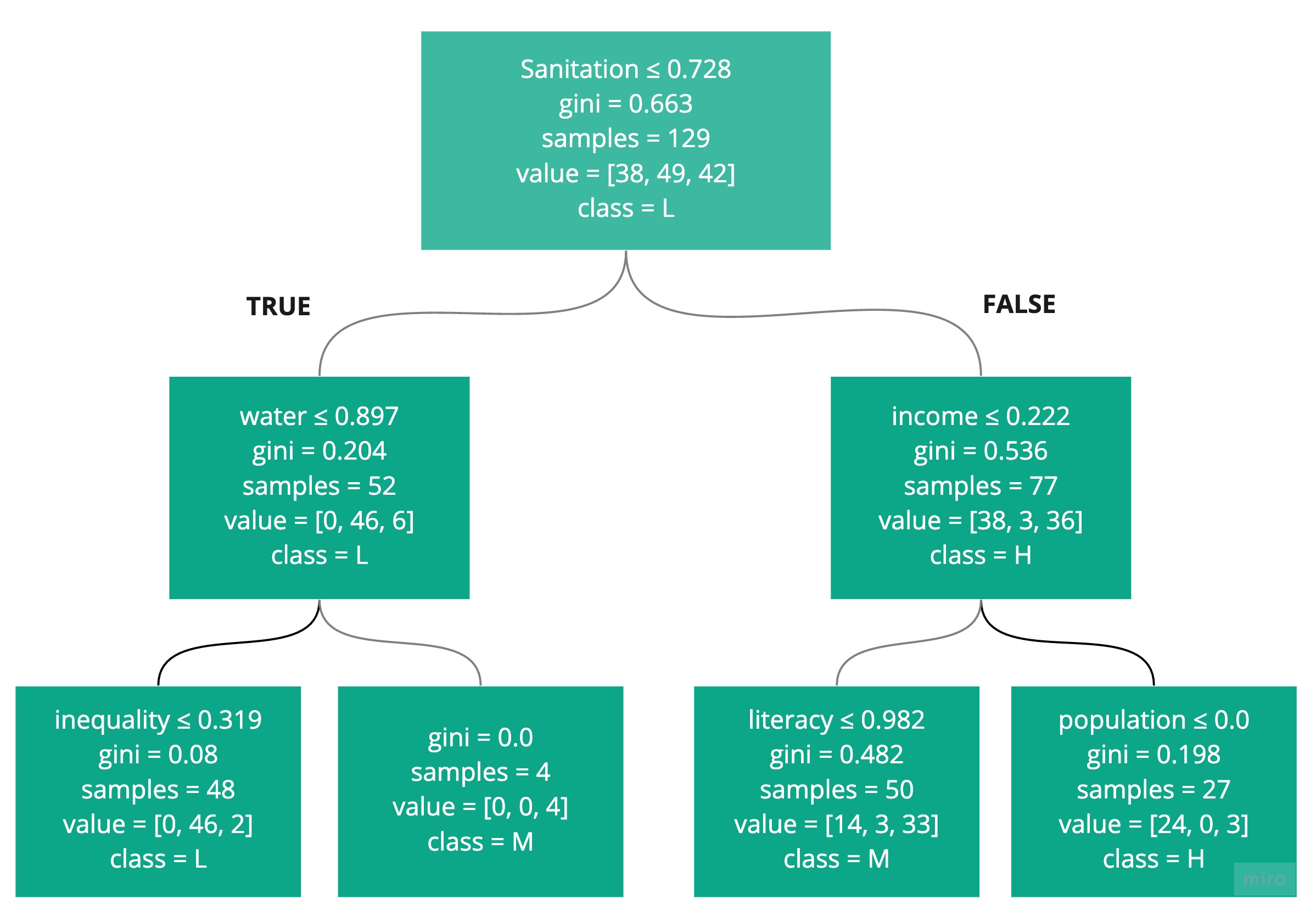

The feature importance, shown below, looks at each feature and determines the importance it plays in the decision tree construction. It tells you the total reduction in the Gini. As you can see, sanitation was the most important, followed by happiness. This tells us nothing about which class each feature helps to predict - just its impact on the overall classification task. 

The  decisionTreeSummary()  function can be found in  functions.py.  It uses the  feature_importances_  attribute of the DecisionTreeClassifier.

decisionTreeSummary(model_dt, X.columns)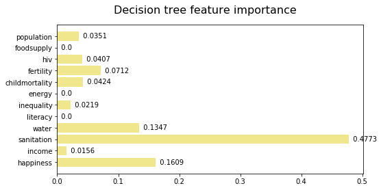

Logistic Regression

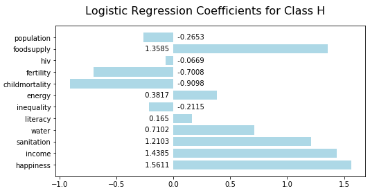
Examine the coefficients for logistic regression. These effectively define the shape of the sigmoid curve that models the data. There is a coefficient for each feature. The sign and magnitude indicate the degree to which features influence the classification decision. Look at the following visualization: 

The  logisticRegressionSummary()  function can be found in  functions.py.  It uses the  coef_  attribute of the LogisticRegressionClassifier.

logisticRegressionSummary(model_lr, X.columns)

Looking at the first chart, you can see that high food supply, income, and sanitation are indicators of high life expectancy:

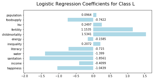
Low sanitation is the most significant indicator of low life expectancy:

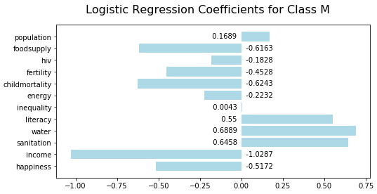
Low income is the most significant indicator of medium life expectancy:

Recap

• You can choose a machine learning algorithms by building models with multiple algorithms and seeing which one performs the best.

• Measure the performance of a classification model using an accuracy score.

• Iterate to improve model performance.

• Inspect the feature importance values to understand which features are most significant in a decision tree model.

• Inspect the coefficients to understand which features are most significant in a logistic regression model.

 In the next part, we will build a regression model! But for now, it's time to test your knowledge!