Understand the Decision Trees Algorithm
Decision Trees
In Part 1, we used the following training dataset to build a model that could predict happiness from lifeexp and unemployment:
| lifeexp | unemployment | happiness |
0 | 77.6 | 6.09 | Low |
1 | 75 | 3.24 | Low |
3 | 71.9 | 1.53 | Low |
4 | 61.8 | 7.52 | Low |
6 | 81.4 | 1.43 | High |
8 | 80.7 | 1.36 | High |
9 | 75.7 | 4.96 | High |
11 | 77.5 | 0.06 | High |
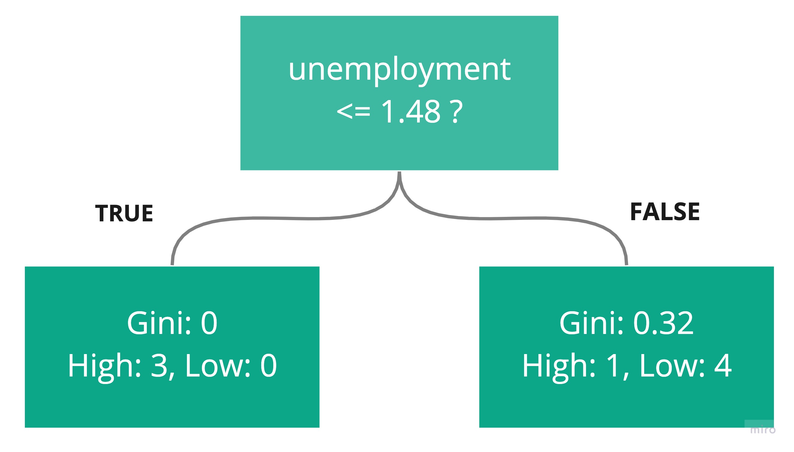
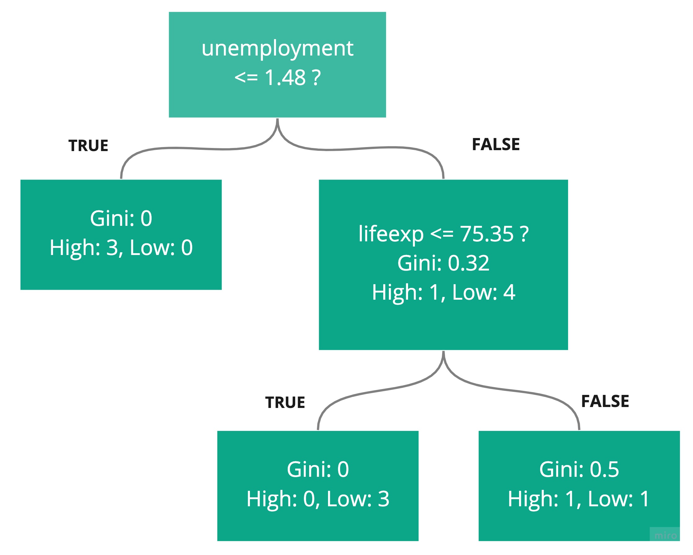
We used the sklearn algorithm, DecisionTreeClassifier, which constructed the following decision tree to make these predictions:
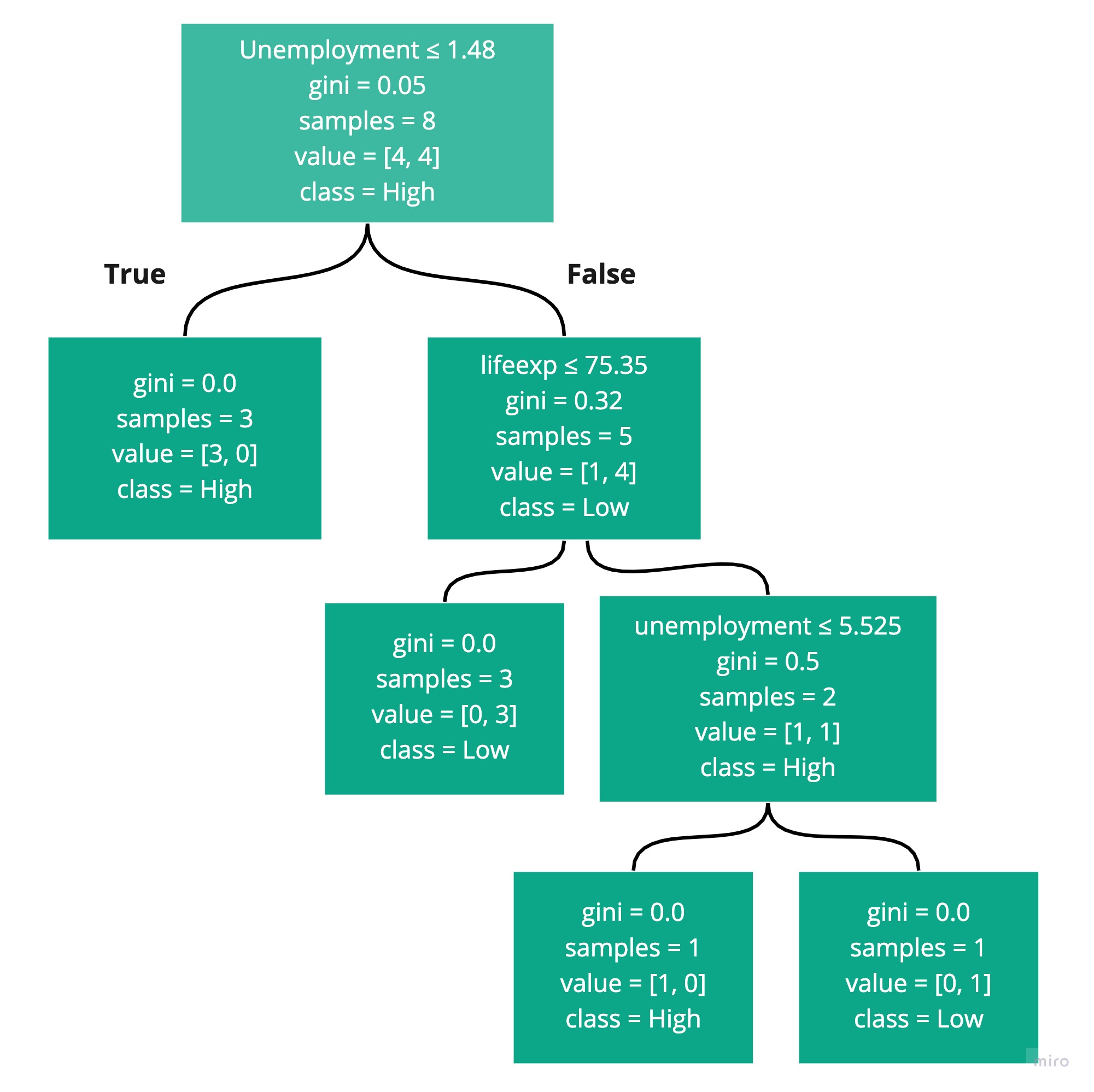
This raised two good questions:
What is Gini?
How did sklearn come up with the rules, and specifically, the boundary values like 5.525?
The time has come to tackle these questions! You don't have to understand all the detail here to successfully use decision trees in Sklearn. But I’m sure you are an inquisitive person and would like to know how this magic works, right? ;)
Gini
The Gini coefficient, or Gini index, measures the level of dispersion of a feature in a dataset.
If you were to plot the cumulative income of the people in a society, starting at 0, then adding the lowest paid person, then the next lowest paid, and so on, until you got to the highest paid person, you would get a chart with a line starting at 0, and increasing to the total income of the entire society.
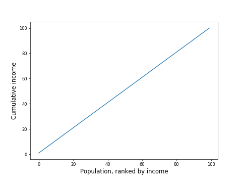
Imagine a society where everyone had the same income. If you plot the cumulative income as described above, you would expect a chart like this, with a straight line from 0 to the total population income:
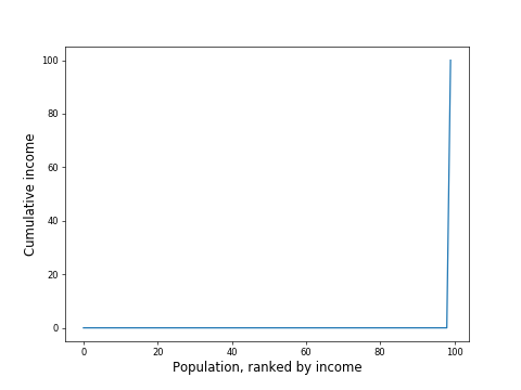
However, if you had a society where everyone earned 0 except one person who earned the entire society's income, you would get a chart like this:
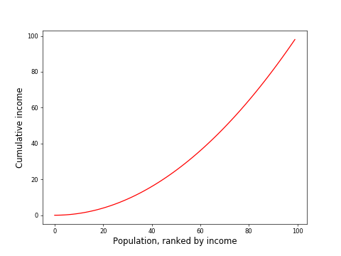
In most real-life societies, the situation would lie somewhere in between the above extremes:
Let's bring the ideal line (blue) and real-life line (red) together:
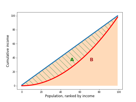
If you compute the area between the curve and the ideal line (area A, hatched in green), and divide by the area below the ideal line (area B, in pink), you get the Gini coefficient.
In the following explanation, we will use Gini to help decide which of the many possible rules to choose from.
Decisions, Decisions
When constructing a decision tree, work from the top down. The boxes are called nodes. The top one is called the root. The nodes at the bottom, which have no nodes below them, are called leaf nodes.
So, the first task is to work out what questions to ask at the root node. Each question is made up of two parts: the feature and the threshold value. Sklearn decided that this should be the first question:
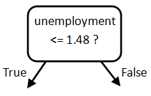
Why did sklearn choose unemployment and not lifeexp? And how did it decide on 1.48 as the split point?
Answer: It computes the Gini coefficient of the original data. It then computes it for data split at every possible threshold for every possible feature! Then it sees which split point reduces the Gini by the greatest amount.
The Decision Tree Algorithm
Here's how the decision tree classifier algorithm proceeds.
Compute the Root Node Gini
First, it computes the happiness Gini of the original data. If all countries had the same happiness, the happiness Gini would be 0. Because there are four high happiness countries, and four low happiness countries (an even split), the initial happiness Gini is 0.5.
Find all the Candidate Root Node Rules
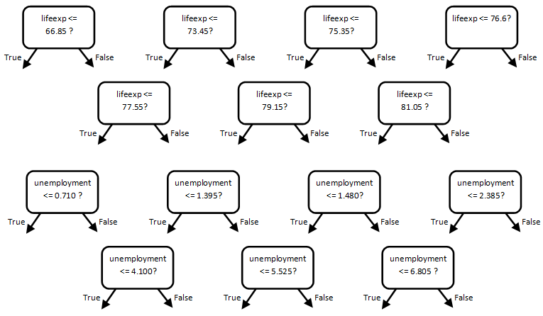
The algorithm starts with the first feature, in this case, lifeexp. It sorts the data by lifeexp and computes the candidate split point between each pair of points by taking the mean of the two points:
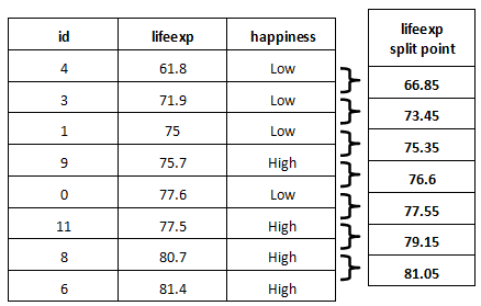
These are all the potential split points for lifeexp.
It repeats the same for the next feature, unemployment:
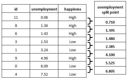
These are all the potential split points for unemployment.
Here are all the potential rules for the root node:
Compute the Happiness Gini for the Result of Each Candidate Split
Each rule will split the countries into two groups. You can compute the happiness Gini for each of these groups.
A feature and threshold that divided the countries into the four low happiness countries on the left, and the four high on the right, would be the perfect rule!
On the left-hand side, all the countries have the same happiness. They are equal. On the right-hand side, all the countries have the same happiness. They are also equal!
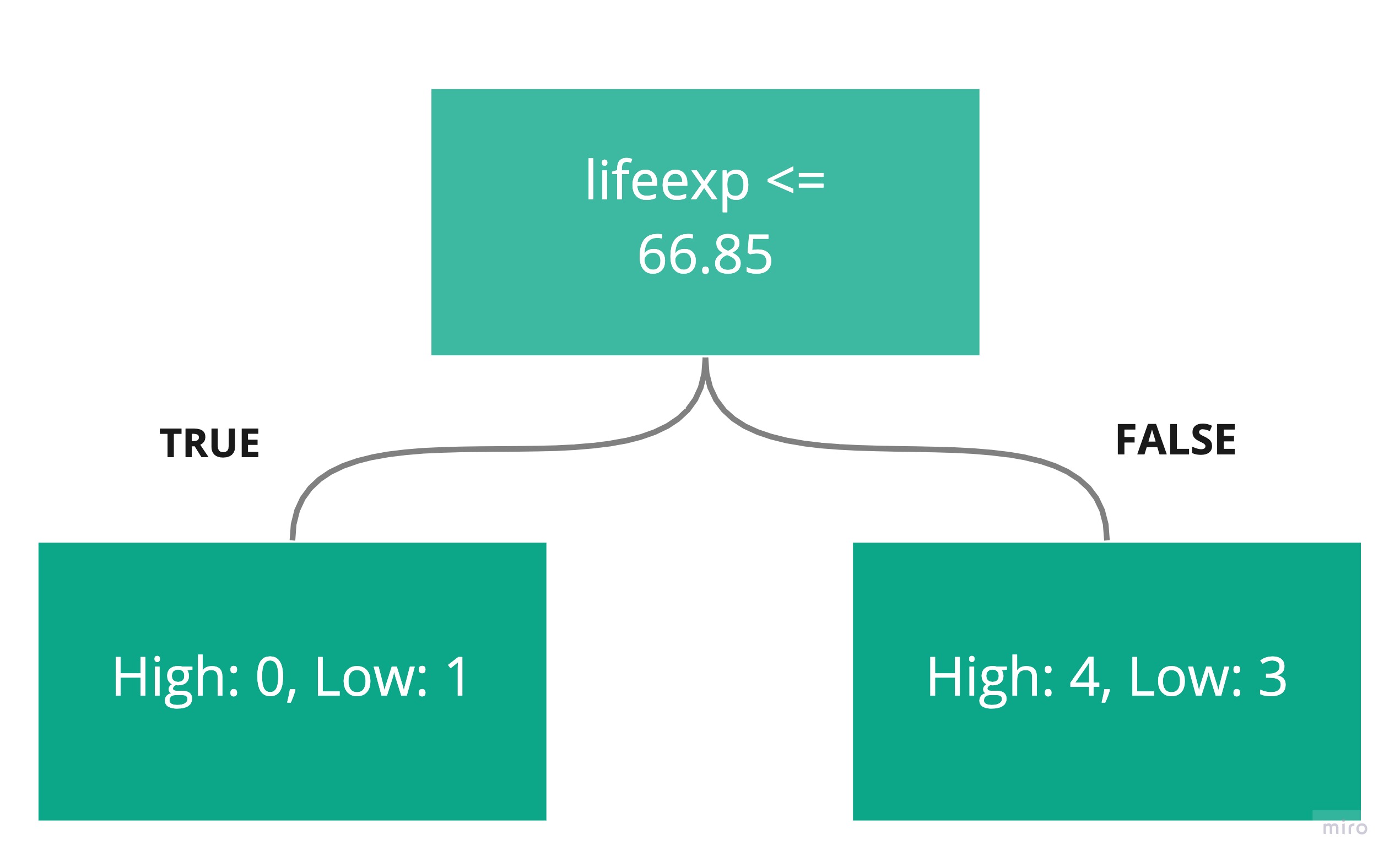
Let’s walk through the computation of the Gini values for the following candidate rule:
First, count the number of high and low happiness values below and above the threshold. Here are the sample points, sorted by lifeexp, and split at the candidate threshold of 66.85:
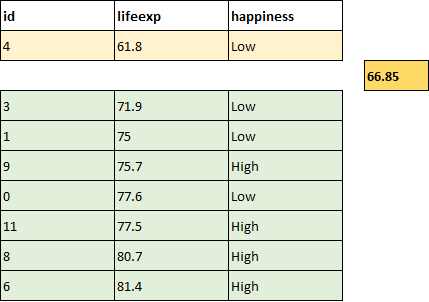
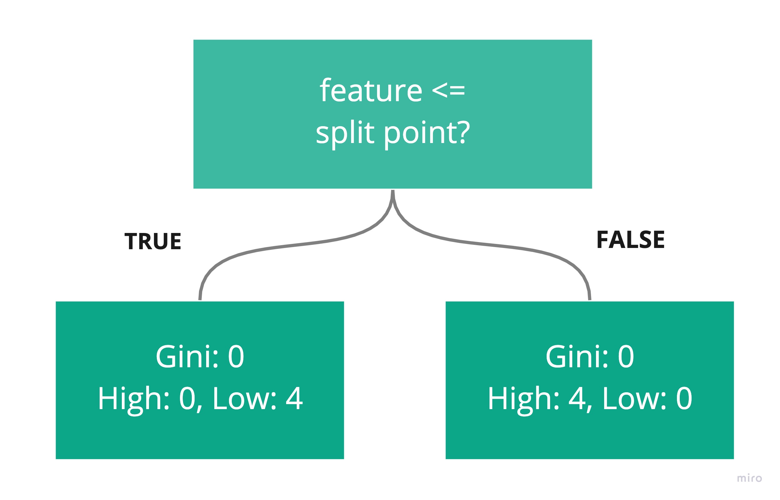
Here is what the rule would look like after the split, with one country below the threshold (in yellow), and seven above it (in green):
Compute the Gini for each side using the following formula:
p(High) is the probability of observing high. On the left-side box, this will be 0. On the right-side box, this will be 4/7.
p(Low) is the probability of observing low. On the left-side box, this will be 1. On the right-side box, this will be 3/7.
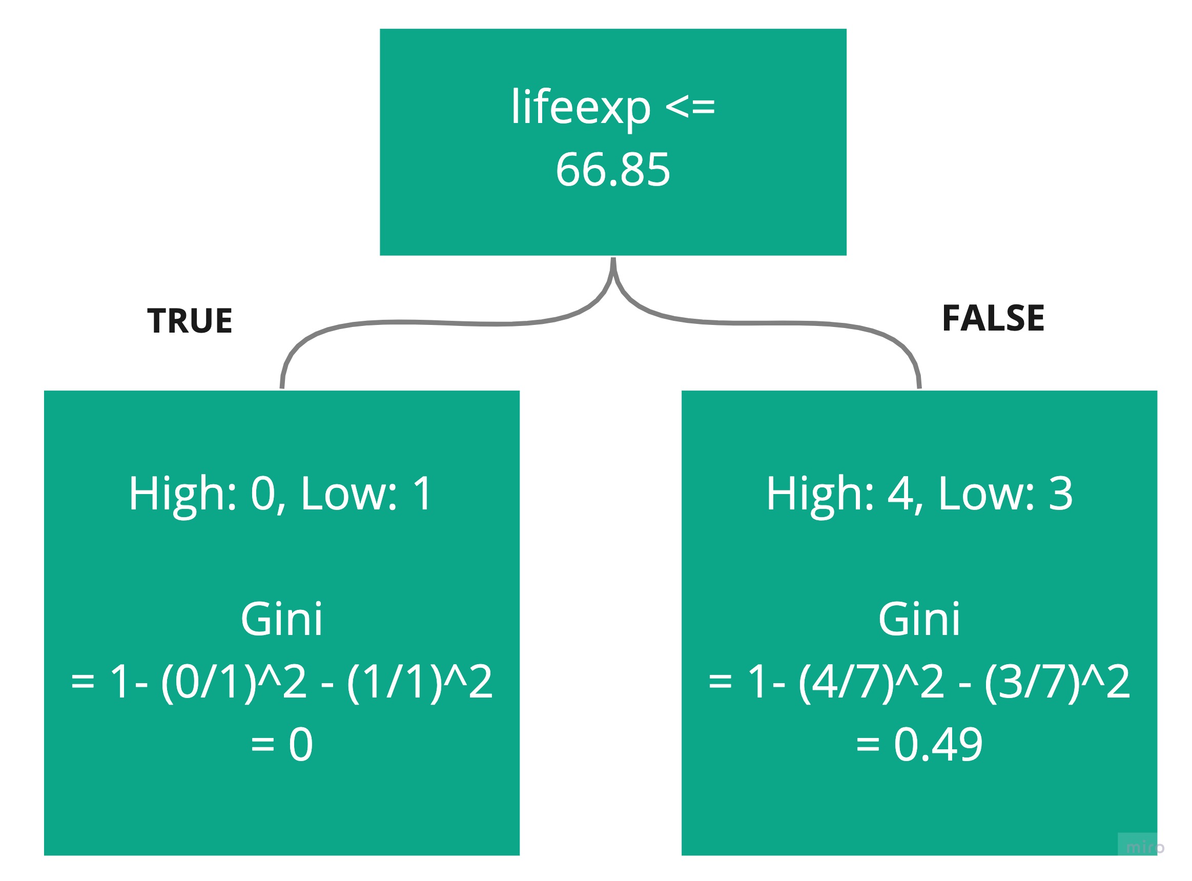
Compute the overall Gini for both sides by weighting each (0 and 0.49) with the number of countries on each side (1 on the left, 7 on the right, 8 in total):
Overall Gini = 1/8 * 0 + 7/8 * 0.49
= 0.43
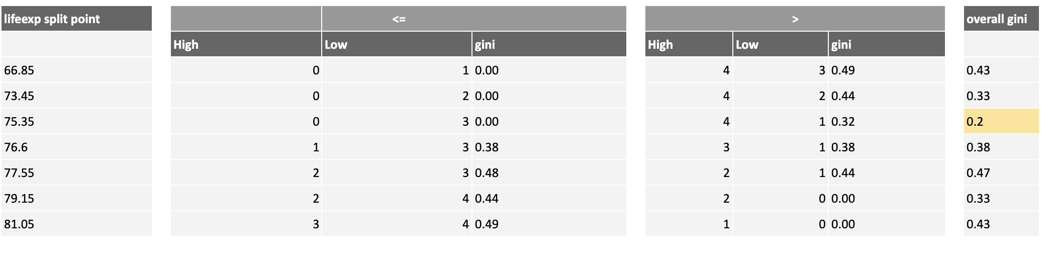
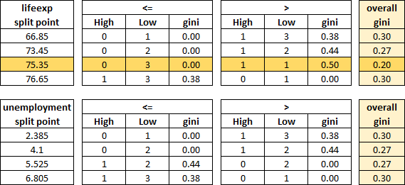
In the same way, compute the overall Gini for the other lifeexp thresholds, highlighting the one that generates the lowest overall Gini in dark yellow:
Compute the overall Gini for the unemployment thresholds, highlighting the threshold that generates the lowest overall one in dark yellow: 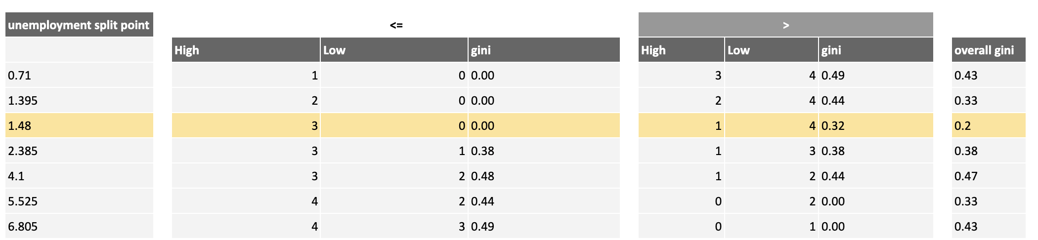
Based on this analysis, there are two possible best choices for the root node rule, both with a Gini of 0.2, which are the yellow rows highlighted above. Because they have the same Gini, you can choose one at random:
We have found the rule that best splits the countries into high and low happiness!
Compute the Next Level Rule
At this point, the left-hand side contains just these high happiness countries, and therefore, has a Gini of 0. There is no more work or sorting to do on this side.
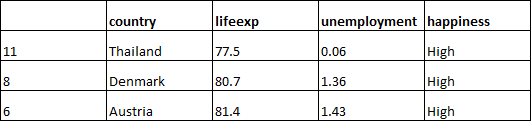
The right-hand side still has a mix of high and low happiness countries.
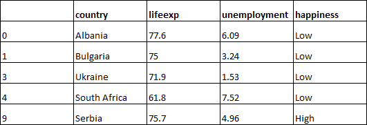
There is still some sorting to do here. So take the countries that have fallen into that node and repeat the above process:
Find all the candidate rules for splitting the remaining countries.
Compute the happiness Gini for the result of each candidate split.
Choose the rule that best reduces the overall Gini.
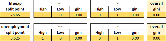
Here is the result of that process for the second rule:
The best rule, which reduces the Gini of those countries the most, is to split lifeexp at 75.35.
Let's now introduce a new rule into the decision tree:
The left-hand side of this rule gives a Gini of 0, so we don't need to do more. On the right-hand side, there are only two countries to split. Applying the same process again gives the following overall Gini calculations:
Both end up with a Gini of 0, so either of the splits would work, and we can add another rule to the decision tree:
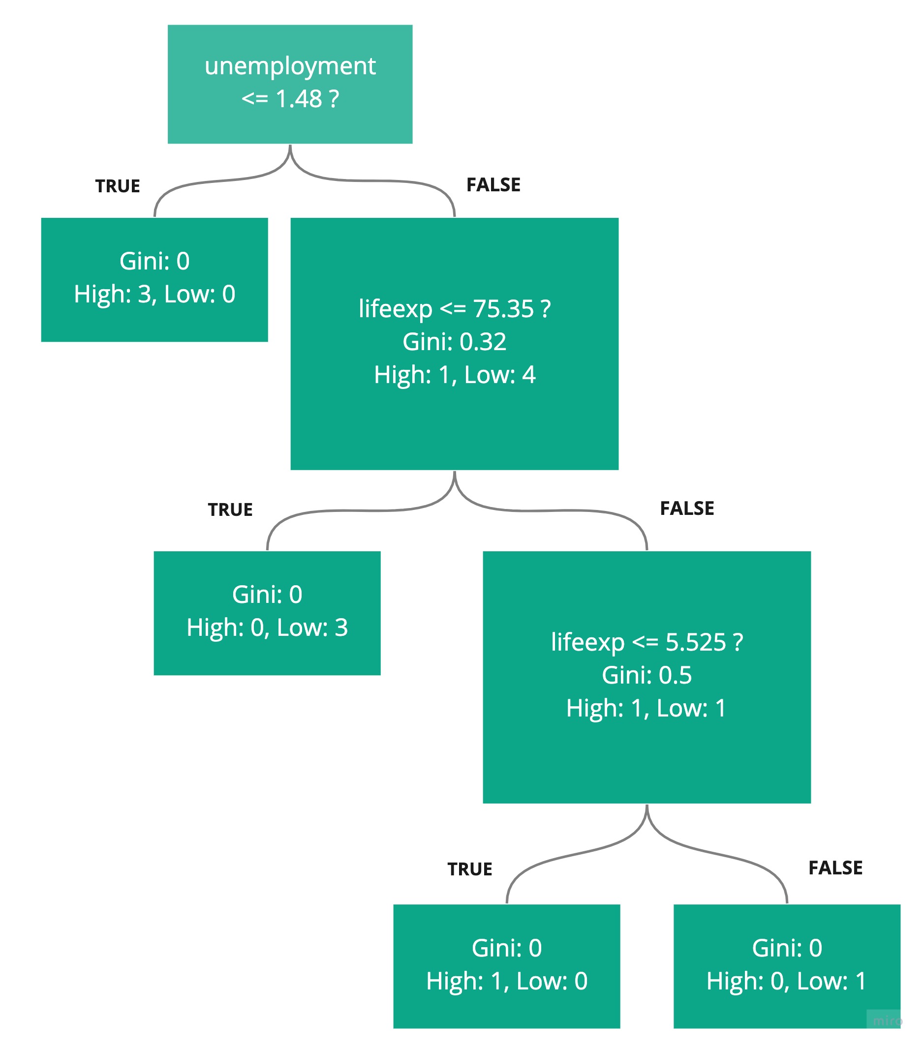
All the data is sorted into leaf nodes with an overall Gini of 0. Our job is done!
Recap
The Gini coefficient, or Gini index, measures the level of dispersion of a feature in a dataset.
A Gini of 0 for a feature signifies a sample where every data point has the same value for that feature (perfect equality).
A Gini approaching 1 for a feature signifies a large sample where one individual is different from all the others (perfect inequality).
Decision trees can be constructed by finding rules that split unequal groups into groups that have a lower overall Gini.
In the next chapter, we will take a look at the logistic regression algorithm.
