Get to Grips with How Principal Component Analysis Works
What is PCA?
Principal Component Analysis (or PCA) is a dimensionality reduction technique. We can use it to transform a large set of variables into a smaller set whilst preserving as much information as possible. In other words, we try to capture the essence of the data with fewer variables.
Why do we need it?
You may wonder why we need to reduce the number of variables at all. Why not just use all of the variables?
A smaller number of variables is easier to work with and can be processed faster.
It can be used to reduce noise in the data, i.e. dimensions which add little to the explanation of the underlying data.
It is also easier to visualise data when we have fewer dimensions (visualising two dimensions is easier than visualising 10 dimensions).
A visual analogy
It may be tricky to imagine how we can reduce data without losing information. How do we choose what variables to reduce, and how much do we reduce them by? And what does "reduce" even mean?
Imagine trying to take a picture of a lamp for a product catalogue. You would want the best angle - the one that shows the maximum amount of information about the lamp, right? So you set up your studio and take test pictures from various angles. You may end up with a set of test images such as the ones below.
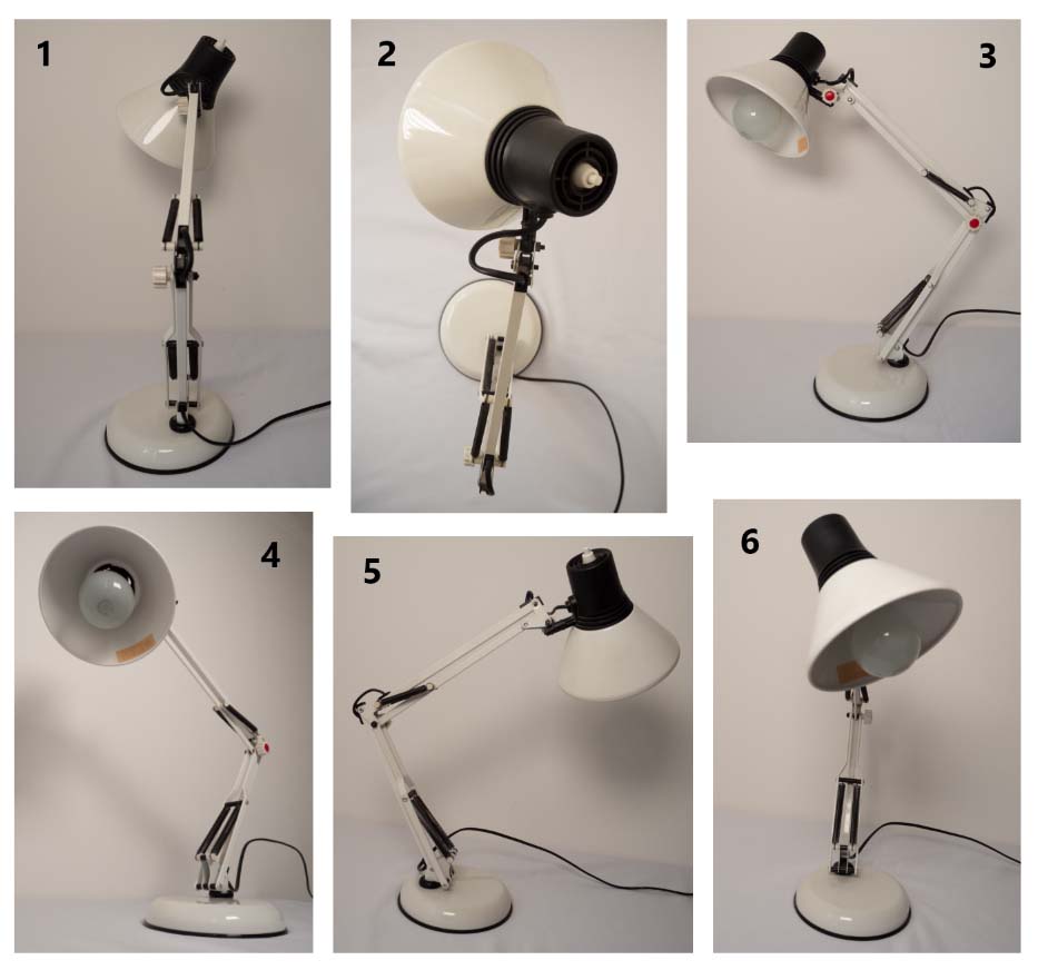 All of these images are transformations of the three-dimensional lamp to a two-dimensional picture of a lamp. In reducing the lamp from 3 dimensions to 2 dimensions, we have certainly lost some information, but in some cases we have lost more than in others. There is an optimal transformation that really preserves the best detail of the lamp.
Which image would you choose for the catalogue?
How PCA works
So we've seen a visual example. But how does this work with a data set? Let's start with an example in two dimensions, which we will then reduce to one dimension. Here is a scatter plot of the heights and weights of 30 people:
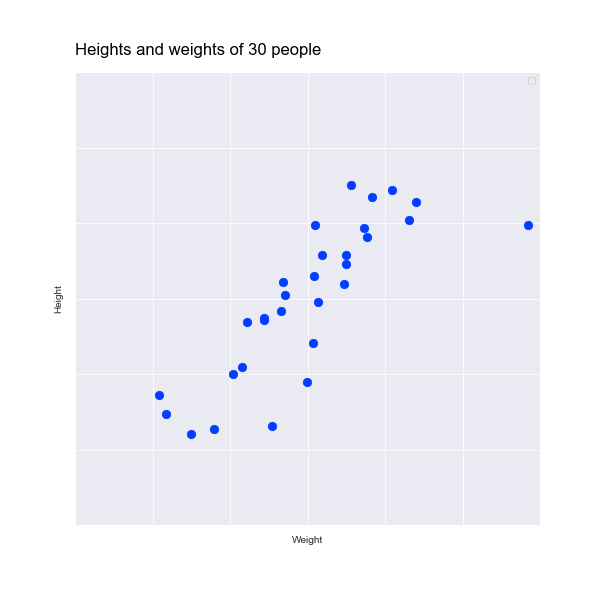
To reduce this to one dimension our aim is to find a single line of points (i.e. one dimension of data) that preserves as much of the variance in the data as possible.
But how do we do this?
We could just eliminate the height dimension, as shown in the animation below:

But this isn't great, as we have lost all information about the height!
Similarly, if we just remove the weight dimension we lose all information about the weight, which you can see in the following animation:
In fact, PCA starts by finding the mean point in the data. In our scatter plot, this is the point at the mean of the weights along the X axis and the mean of the heights of the Y axis. This is marked by an X in the animation below.
PCA then finds a line that passes through the mean point. Of course, there are several lines that pass through this point, as illustrated by the green lines in the animation. So, which one do we choose?
When we map the data points to the line, we preserve information about both the weight and height dimensions:

This line of points represents the original points on a new dimension, which we call Principal Component 1, or PC1. It represents not the weight or the height but a combination of the two. More than that, it's the combination that best represents the variance in the data, helping us preserve as much information as possible when we reduce the weight and height to a single dimension.
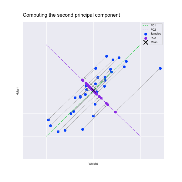
As you can see, the dots are spread out a little above and a little below the line. If we draw another line at right angle to the first one we can also map the points to that line. This gives us another new dimension, Principal Component 2, or PC2:
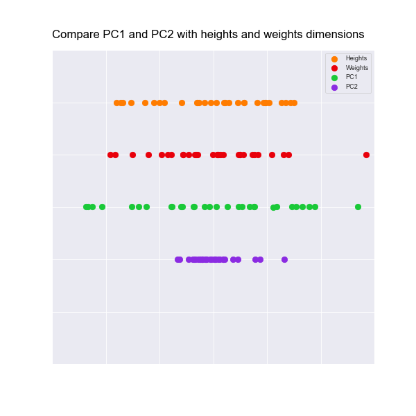
If we rotate these set of points to the horizontal, we can compare the spread of the points with the spread for just the weight and height. Below you can see that PC1 has more variance than either the weight or height alone. It's captured the essence of both. PC2 has less variance than the others, because the variance has been "pushed" onto PC1:
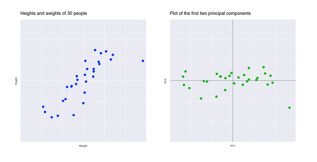
It's worth pausing a moment to understand what PCA has actually done. We can plot PC1 against PC2 using a scatter plot to help our understanding:
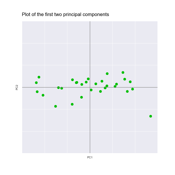
All we have actually done is find the optimal way to rotate our original data so that most of the variance (i.e. the spread) is captured on the horizontal axis. The second image below, which represents our principal components, is just a rotation of the first image, which represents our original data:
Scaling to 3 or more dimensions
What if we add a third dimension to our data?
For example, we could add the person's age to all the data points. We would now need to plot the data in a 3D plot to have a "cloud" of data points. To carry out PCA we would rotate this 3D cloud freely to find the line that passes through the cloud in the optimal way, so that the distance from all the data points to the line is minimized. This is PC1. We then find another line, at right angles to PC1, which again captures the variance best. We can do this by rotating this cloud, but only around the PC1 axis. This is like rotating a piece of chicken on a barbecue spit. Once we find the optimal rotation angle we have PC2. Finally, we select the line that is at right angles to PC1 and PC2. There is only one line that meets this condition and this is PC3.
Moving to 4 or more dimensions is difficult to visualise, but the maths still works! We could have 100 dimensions and compute PC1, PC2 all the way up to PC100.
Using the PCA results
Once we have transformed our data using PCA we have a number of principal components, PC1, PC2, all the way up to PCn. The aim of PCA is to reduce the number of dimensions. Because the dimensions are ordered by their ability to capture the essence or variance in the data, we can keep the first few and throw away those at the end that don't add much to our understanding of the variance of the data.
Terminology
It's useful to be aware of some of the terminology that is used by mathematicians when discussing PCA. Don't worry if this doesn't make too much sense at the moment. You can come back to it when you are more comfortable with applying PCA with code (which we will do soon) and do some further reading if you want to understand the mathematics behind PCA in more detail.
The set of numbers that define a point in our data set is called a vector. For example here is a two-dimensional vector representing the height and weight of an individual:
(68, 175)
We could also represent it as a table:
Weight | Height |
168 | 175 |
Here is a three-dimensional vector representing the height, weight, and age of an individual:
(68, 175, 44)
Again we can represent it as a table:
Weight | Height | Age |
68 | 175 | 44 |
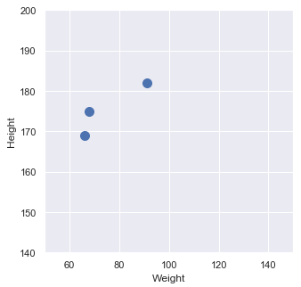
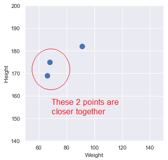
Vectors represent points in a space and a space has dimensions. Here are 3 two-dimensional vectors, shown as a table:
Weight | Height |
68 | 175 |
66 | 169 |
91 | 182 |
They sit in a two-dimensional vector space:
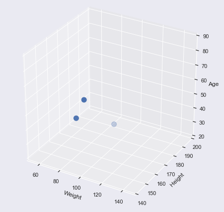
Here are 3 three-dimensional vectors:
Weight | Height | Age |
68 | 175 | 44 |
66 | 169 | 34 |
91 | 182 | 27 |
They sit in a three-dimensional vector space.:
More generally, a vector of length n sits in an n-dimensional vector space.
We can compute the length of a vector by computing the square root of the sum of squares, which is just Pythagoras Theorem.
We can compute the distance between two vectors.
The length of vectors and distance between vectors are frequently calculated to determine how related data points are. For example, in the 2D vector space above we can clearly see that two of the points are closer to each other than to the other point:
We can also do this in 3D vector space:
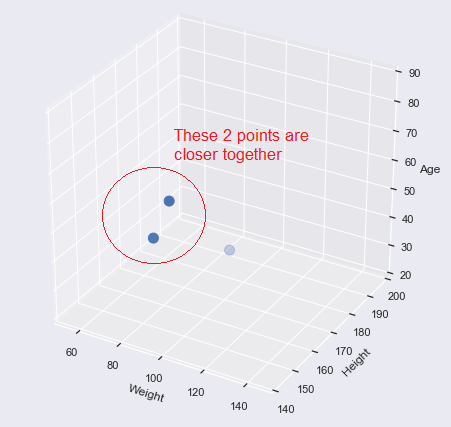
And the good news is that we can also compute distance in n-dimensional space. This is really great news as we can use it to find relationships between data samples with any number of variables! For example, in PCA we can use it to find the optimal lines through the set of vectors in the vector space (remember that the optimal line is the one that minimises the sum of the distance from the data points to the line).
We use Principal Component Analysis to perform dimensionality reduction. PCA uses a technique called Singular Value Decomposition.
The dimensions in an n-dimensional space are all orthogonal to each other. This essentially means they are at right angles to each other. Intuitively this makes sense in 2 or 3 dimensions, but mathematically this also applies to 4 or more dimensions.
In the next chapter we will get going with writing some Python code to carry out a PCA.
Recap
PCA uses vector maths to calculate some properties of space that we find very intuitive in 2D and 3D.
Even though we can't visualise four or more dimensions, the vector maths still works and provides ways to determine how related data samples are and which variables best describe those data points.
