Carry Out a K-Means Clustering
In the previous chapter we learned about how the k-means algorithm finds groups of similar data points in a sample. Let's write some Python code using Sklearn to carry out a k-means clustering. We will use the same Times Educational Supplement University rankings data that we used in the PCA exercise.
Loading, Cleaning and Standardizing the Data
As with our PCA exercise, we need to first load, clean and standardize our data:
# Import standard libraries
import pandas as pd
import numpy as np

# Import the kmeans algorithm
from sklearn.cluster import KMeans

# Import functions created for this course
from functions import *
Load the data set:
# Load the data from the csv file into a Pandas Dataframe
original_data = pd.read_csv('world_university_rankings_2016.csv', index_col='university_name')
original_data.head()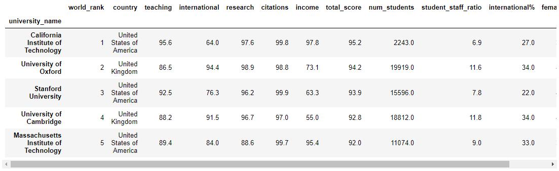
K-means can only work with quantitative data, so we will remove country.
In addition, we will remove the total_score and world_rank columns as they are the totals and rank for the table as a whole. We are really interested in analyzing the underlying metrics that contribute to the overall score.
So let's filter our data down to just the remaining columns of interest:
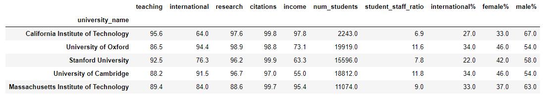
As with our PCA exercise, we will replace nulls with the mean value of the variable:
X = X.fillna(X.mean()) Again, we will apply the standard scaler to scale our data so that all variables have a mean of 0 and a standard deviation of 1.
# Import the sklearn function
from sklearn.preprocessing import StandardScaler

# Standardize the data
scaler = StandardScaler()
X_scaled = scaler.fit_transform(X)
X_scaled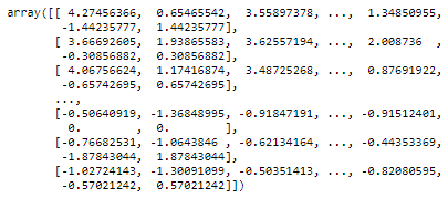
So, thus far we have treated the data in exactly the same way we did for PCA.
Performing a K-means Clustering
Now we can perform the k-means clustering. We will ask for 3 clusters (the n_clusters parameter) and ask for clustering to be performed 10 times, starting with different centroids (this is the n_init parameter). In this way, we can ask the algorithm to give us the best of the 10 runs.
# Create a k-means clustering model
kmeans = KMeans(init='random', n_clusters=3, n_init=10)

# Fit the data to the model
kmeans.fit(X_scaled)

# Determine which clusters each data point belongs to:
clusters =  kmeans.predict(X_scaled)
Let's add a new column, cluster number to the original data so we can see what universities sit in what cluster:
# Add cluster number to the original data
X_scaled_clustered = pd.DataFrame(X_scaled, columns=X.columns, index=X.index)
X_scaled_clustered['cluster'] = clusters

X_scaled_clustered.head()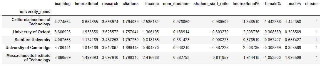
And...That's it! Really! We have performed a k-means clustering on our data. In the next chapter we will analyse the results.
Selecting the Number of Clusters
In the exercise above we decided to create 3 clusters. But why 3? To be completely honest, there was no logic to our choice. So then...how do we work out the ideal number of clusters?
There is no magic number of clusters, but we can use a technique called the Elbow Method to help us with this question.
The Elbow Method runs multiple tests with different values for k, the number of clusters. For each run it records the score, which is a measure of the in-cluster variance (in other words how tight the clusters are). We can then plot the score against the number of clusters. Let's do that with our data:
# Run a number of tests, for 1, 2, ... num_clusters
num_clusters = 50
kmeans_tests = [KMeans(n_clusters=i, init='random', n_init=10) for i in range(1, num_clusters)]
score = [kmeans_tests[i].fit(X_scaled).score(X_scaled) for i in range(len(kmeans_tests))]

# Plot the curve
plt.plot(range(1, num_clusters),score)
plt.xlabel('Number of Clusters')
plt.ylabel('Score')
plt.title('Elbow Curve')
plt.show() 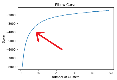
I've added a red arrow to identify the "elbow" in the curve. You can see that the curve rises sharply from 1 up to around 5 clusters but starts flattening out. By about 15 clusters, the curve is very flat and nearly horizontal. What this means is that above around 10 clusters the additional reduction in variance (or increase in the "tightness" of the clusters) is reducing significantly for each additional cluster. So there is little point in choosing more than 10 clusters and the ideal number is probably somewhere between 5 and 10.
Recap
Selecting the number of clusters can be a bit of a guessing game, but the elbow method can be a useful guide
Use the
n_clustersparameter in Python to ask for the number of clusters that you need
