Carry Out a Principal Component Analysis
Introducing our data set
For this chapter, we will be using the Times Educational Supplement university rankings data. This data is published annually and covers over 1,000 universities across the work.

For our convenience, this data has been made available in csv format on Kaggle.
For the purposes of this course I have filtered this down to just the 2016 rankings (the latest available in the above Kaggle dataset).
When doing any data analysis it is important to understand as much about the meaning of the data as possible. Data analysis should not be a purely mathematical exercise! Here are the descriptions of the columns from Kaggle:
world_rank: world rank for the university. Contains rank ranges and equal ranks (eg. =94 and 201-250)
university_name: name of university
country: country of each university
teaching: university score for teaching (the learning environment)
international: university score international outlook (staff, students, research)
research: university score for research (volume, income and reputation)
citations: university score for citations (research influence)
income: university score for industry income (knowledge transfer)
total_score: total score for university, used to determine rank
num_students: number of students at the university
student_staff_ratio: Number of students divided by number of staff
international%: Percentage of students who are international
female%: Percentage of female students
male%: Percentage of male students
Full details of the methodology used to prepare the data can be found here.
Let's start by importing the libraries we need - Pandas and numpy. We will also import a small library of convenience functions used specifically for this course. Feel free to open up functions.py to see what's inside it.
# Import standard libraries
import pandas as pd
import numpy as np

# Import functions created for this course
from functions import *
Now we load the data from the csv file, setting the university_name column as the index column:
# Load the data from the csv file into a Pandas Dataframe
original_data = pd.read_csv('world_university_rankings_2016.csv', index_col='university_name')
original_data.head()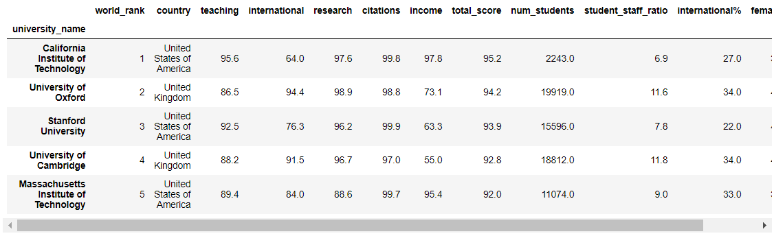
PCA can only work with quantitative data, so we will remove country.
In addition, we will remove the total_score and world_rank columns as they are the totals and rank for the table as a whole. We are really interested in analyzing the underlying metrics that contribute to the overall score.
So let's filter our data down to just the remaining columns of interest:
X = original_data[['teaching', 'international', 'research',
       'citations', 'income', 'num_students', 'student_staff_ratio',
       'international_students', 'female%','male%']]
X.head()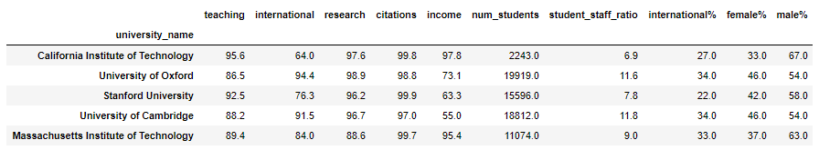
As you will remember if you viewed the previous course in this series, data often contains nulls and we usually need to deal with is in some way, or many of our analyses will fail. Let's see if our data contains nulls by running the info() method on our Dataframe:
X.info()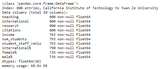
As we can see, there are 800 samples, and for some of the variables (data columns), there are fewer than 800 non-null values. So there must be some null values!
Let's deal with the nulls by replacing them with the mean value for the variable. Obviously, this has risks as far as the data integrity is concerned, but it's a common strategy for dealing with missing values (to read more about other strategies, check out the course Perform an Initial Data Analysis).
X = X.fillna(X.mean()) Standardize the data
Let's take a look at the range of values for the variables we have. We can do this using the describe() method of the Dataframe:
X.describe()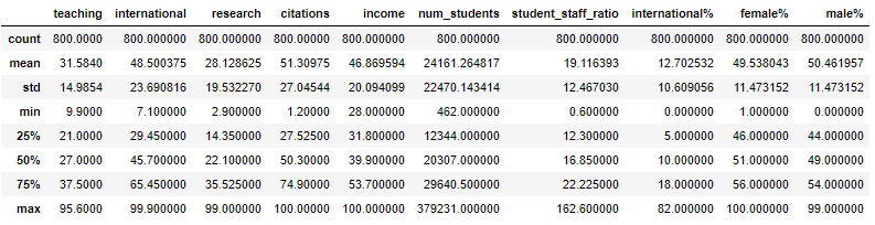
If we look at the min and max values we can see that most of them (teaching, research, citations, etc, ) look like percentage scores. However, num_students has a min value of 462 and a max value of 379,231. Clearly, this is on a different scale to the other variables. If we proceed to carry out a PCA using the data as it stands we would find that num_students would be far too strongly represented in the result.
To address this we need to carry out a common data pre-processing task called scaling. More specifically, we will be standardising the data. That is to say, we will transform all our data so that all variables are on the same scale. Or to put that mathematically, all variables will have a mean of 0 and standard deviation of 1.
Let's apply the standard scaler:
# Import the sklearn function
from sklearn.preprocessing import StandardScaler

# Standardize the data
scaler = StandardScaler()
X_scaled = scaler.fit_transform(X)
X_scaled
If you are unsure exactly what the StandardScaler has done, it's worth plotting the data before and after this technique was applied. Before the transformation, plotting the distribution of the values of each variable except for num_students looks like this:
X1 = pd.DataFrame(X,columns=X.columns)
X1.drop('num_students', axis=1,inplace=True)
X1.plot(kind='density',sharex=True,figsize=(12,5),layout=(10,1))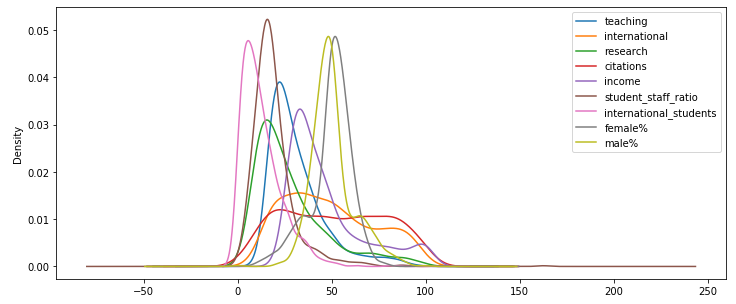
The distribution for num_students is on such a different scale that we need to plot it separately:
X2 = pd.DataFrame(X,columns=X.columns)['num_students']
X2.plot(kind='density',sharex=True,figsize=(12,5),layout=(10,1))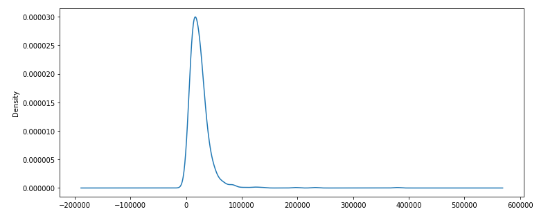
After standardisation we can plot all distributions on the same chart:
pd.DataFrame(X_scaled,columns=X.columns).plot(kind='density',sharex=True,figsize=(12,5),layout=(10,1)) 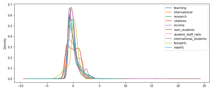
As you can see, all the distributions are now centered around the 0 value and have a similar spread. The variation in the data is still preserved (you can see that the shape of the density plot lines remains similar to the original plot for each variable).
So, now we have removed the bias caused by different scales we can proceed to...
Perform PCA
So, let's get on to the main event! First we need to import PCA from sklearn and select the number of principal components we will return. We will ask for 10 components, which is the maximum we can ask for because we have 10 variables. Next, we create the PCA model, and fit the model with the standardized data. Here is the code to perform a PCA on our standardized data:
# Import the PCA function from sklearn
from sklearn.decomposition import PCA

# Select the number of principal components we will return
num_components = 10

# Create the PCA model
pca = PCA(n_components=num_components)

# Fit the model with the standardised data
pca.fit(X_scaled)
PCA(copy=True, iterated_power='auto', n_components=10, random_state=None, svd_solver='auto', tol=0.0, whiten=False)
That's it! Now, inside the PCA model is everything we need to know about new PCA vector space.
In the next chapter we will take a look inside the PCA model and understand how to interpret it.
Recap
The steps to carrying out a PCA:
Import the necessary libraries
Load the data from the CSV file
Remove variables that you don't require for your analysis and deal with null values
Standardize the data
Perform a PCA!
