Perform an Initial Data Analysis

We are now going to cleanse the data set we saw in the previous chapter. We will illustrate this in Python.

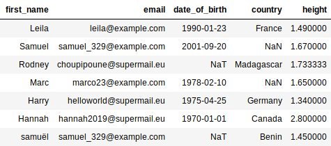
We will begin by loading the sample persons.csv (which you can find here) into a variable we will call  data . This variable will therefore be a dataframe.

Next, we will comb through each of the columns looking for errors, correcting them, and updating the columns accordingly. Whether you are working in Python or R, updating a column in a dataframe is performed like this:

data["name_column"] = new_column

Here, we want to replace the values of the  name_column  column (or variable). If the

dataframe has 7 lines, then  name_column  column will contain 7 values. To replace them,

new_column has to be a list of 7 values.

Use the Apply and Map Methods

We still need to know how to populate  new_column . In fact, this will be calculated from

name_column  . We need to comb through each  name_column  value, verify whether it is correct or not, and correct it as needed. For this, we use the  apply  method. This method applies a function to each value of a dataframe column. Alternatively, we can use the  map  method, which is (more or less) equivalent. It applies a check / correct function to each value:

import pandas as pd # the Pandas Libraries is imported and aliased 'pd'.

def lower_case(value): 
    print('Here is the value I am processing : ', value)
    return value.lower()

data = pd.DataFrame([['A',1],
                     ['B',2],
                     ['C',3]], columns = ['letter','position'])

new_column = data['letter'].apply(lower_case)
new_column = new_column.values
print(new_column)
data['letter'] = new_column
print(data)

On line 7, we create our dataframe. This is a table with 2 columns ('letter' and 'position') and 3 rows. On line 3, we create a function named   lower_case  , which takes as a parameter a  value  , displays it (line 4), converts it to   lower case  (line 5), then returns it. Next, we select the  letter column  from data , call the  apply  method, and specify that each of the values be sent, one at a time, to the  lower_case  function (line 13).

On line 11,  new_column  is “column” type (because the   apply  method returns a column). In the Pandas library, the exact column type is  Series  . To obtain the values for this column in the form of a list, we call new_column.values (line 12). Here is what the program will display:

Here is the value I am processing :  A
Here is the value I am processing :  B
Here is the value I am processing :  C
['a' 'b' 'c']
  letter  position
0      a         1
1      b         2
2      c         3

Lines 1 to 3 display what the  lower_case  function is doing; line 4 displays the processing result, that is, the three lower-case letters; and the other lines display the dataframe in which the letter column has been updated to lowercase!

Attack!

Load the Data

Begin by downloading the CSV file that corresponds to the example in previous chapters (provided at the beginning of the chapter), then load it using these lines of code:

# importation of libraries we will need
import pandas as pd
import numpy as np
import re

# loading and display of data
data = pd.read_csv('persons.csv')
print(data)

Process Country Names

As you have no doubt understood, we will need one function per process. Let’s forget  lower_case , and write a function that verifies whether the countries in the  Country column are correct. To do this, we need a list of valid country names:

VALID_COUNTRIES = ['France', 'Madagascar', 'Benin', 'Germany'
                  , 'Canada']
                  
def check_country(country):
    if country not in VALID_COUNTRIES:
        print(' - "{}" is not a valid country, we delete it.' \
            .format(country))
        return np.NaN
    return country

Here, if the country in the  country  variable is not on the  VALID_COUNTRIES  list, we display that message on lines 6 and 7. Then, we return  np.NaN  , which is the value used by the Numpy and Pandas libraries to indicate that a value is unknown. It is roughly equivalent to None.

Otherwise, if the country is valid, we simply return it (line 9)!

Process Emails

Now it’s the emails’ turn! The problem with this column is that there are sometimes two email addresses per row. We only want to take the first one. We will therefore create the  first  function:

def first(string):
    parts = string.split(',')
    first_part = parts[0]
    if len(parts) >= 2:
        print(' - There are several parts in "{}", we are only keeping {}.'\
            .format(parts,first_part))  
    return first_part

When there is more than one email per line, they are separated by commas. We therefore separate the character string of the  string  variable according to commas using the split method (line 2). The result is a list with as many items as there are email addresses; this list is placed in the  parts  variable.

Since  parts  contains at least one item, we place it in the  first_part  variable. Then we count the number of items in  parts  using the  len  function. If there are at least two items, we display the message shown on lines 5 and 6. Finally, we return  first_part  , which contains the first email!

Process Heights

Here we will have two functions:  convert_height , which will convert character strings of type 5'4  to decimal numbers, and  fill_height  , which will replace the missing attributes with the average height (mean) of the sample.

def convert_height(height):
    found = re.search('\d\.\d{2}m', height)
    if found is None:
        print('{} is not in the right format. It will be ignored.'.format(height))
        return np.NaN
    else:
        value = height[:-1] # the last character is removed: 'm'
        return float(value)

def fill_height(height, replacement):
    if pd.isnull(height):
        print('Imputation by the mean : {}'.format(replacement))
        return replacement
    return height

 The first function is a little more elaborate. You can just blindly trust it, or you can attempt to pierce its veil of mystery by reading the Take It Further section at the end of this chapter. :magicien:

Let’s move on to the second function. Ah! It takes two parameters:  height and  replacement . The first is the height, as usual. The second is the value to be returned if there is a missing attribute. Line 11 checks to see whether the  height  value is missing (None, NaN or NaT). If it is, we return the replacement value (line 13). Otherwise, we return  height  .

Apply All Functions

Now that these functions are defined, let’s execute them! At the end of your program, add the following:

data['email'] = data['email'].apply(first)
data['country'] = data['country'].apply(check_country)
data['height'] = [convert_height(t) for t in data['height']]
data['height'] = [t if t<3 else np.NaN for t in data['height']]

mean_height = data['height'].mean()
data['height'] = [fill_height(t, mean_height) for t in data['height']]
data['date_of_birth'] = pd.to_datetime(data['date_of_birth'], 
                                           format='%d/%m/%Y', errors='coerce')
print(data)

 Do you recall the syntax for updating a column we saw at the very beginning of this chapter? We use it here in lines 1 to 4, 6 and 7. You are familiar with the syntax used in lines 1 and 2. However, for lines 3, 4 and 6 you may need to refresh your memory about list comprehensions. If this term means nothing to you, scroll down to the Take It Further section.

What else is there left to tell you? You have all of the essentials. Well, except for a few minor details:

•  h if h<3 else np.NaN  returns  h  if  h  is less than 3, otherwise it returns  np.NaN . This is used to delete heights in excess of 7'0", which are aberrations.

• data['height'].mean()  returns a unique value, which is the mean of all the heights.

• The  date_of_birth column  contains character strings. We convert them to dates, specifying the date format. Character strings that do not conform to this format will be converted in  pd.NaT  (this is the case for Rodney’s date of birth).

Line 9 displays the final result:

Take It Further: List Comprehension

List comprehension is a very practical syntax, because it can be used to write a loop that creates a list, in one line. For example, line 3 of the last bit of code above is equivalent to 4 lines (lines 3 to 6):

data = pd.read_csv('persons.csv')

new_column = []
for t in data['height']:
    new_column.append(convert_height(t))
data['height'] = new_column

Would could very well have used  apply :

data = pd.read_csv('persons.csv')

data['height'] = data['height'].apply(convert_height)

Take It Further: Processing heights

Let’s go back to the function we left behind:

def convert_height(height):
    found = re.search('\d\.\d{2}m', height)
    if found is None:
        print('{} is not in the right format. It will be ignored.'.format(height))
        return np.NaN
    else:
        value = height[:-1] # the last character is removed: 'm'
        return float(value)

Normally, Pandas automatically detects whether a column from a CSV file contains numbers or character strings. But here, the Height column contains "m"s (for “meters”). Because “m” is a letter, Pandas considers "1.34 m" to be a character string, not a number! We must therefore convert it ourselves.

So... it’s true that line 2 is hard to understand. It checks to see whether the height is properly formatted, that is, in the form of a number followed by a decimal point, then two numbers, then an "m." Thus, "1.34 m" is correct; "153 cm" is not.

You now hold the keys to understanding the rest of this function. Note that float(value) is used to convert a character string representing a number to... a real number (whose type is “float”)!