Calculate Measures of Central Tendency
In this section, we are going to perform univariate analyses. Univariate analyses focus on only one variable at a time.
Say you need to drive to a job interview located some distance away in another city, and you wonder what time you should leave in order to arrive there by 3:00 p.m. Since you have a lot to do in the morning, you don’t want to leave too early, but you still want to make sure you get there on time.
You aren’t familiar with the route you’ll be taking but, fortunately, a friend of yours drives it every day. He knows it by heart.
"How much time does it take to drive from this city to that city?" you ask.
"It depends on how much traffic there is. Most of the time it takes me 40 to 45 minutes," he answers.
Let’s look at this sentence. Your friend is familiar with the route; he’s driven it perhaps 1,000 times! Each time, he took note (more or less unconsciously) of how long it took. So we have a sample of 1,000, with one continuous quantitative variable: the time it took to drive between the two cities.
Even though, in theory, the trip time can take values of between 0 and infinity, I’m sure you know that these trip times concentrate around a certain value. What you want here is some idea of where (on an axis from 0 to infinity) the trip time values concentrate.
.” The word concentrate contains the word centre, does it not?
Exactly! We have now arrived at the topic of this chapter: measures of central tendency. We’ll look at three such measures, and—guess what!—they all start with the letter M!
Measures of Central Tendency
The Mode
Most of the time, it takes me 40 to 45 minutes.
When your friend said that, he was giving you a measure of central tendency called the Mode.
For qualitative variables, or for discrete quantitative variables, the mode is the most commonly occurring category or value. In our bank statement, the mode of the categ variable is “Other,” because the “Other” category occurs 212 times in the sample, and all of the other categories (“rent,” “groceries,” etc.) occur fewer times.
For continuous quantitative variables, we aggregate values, grouping them into bins (intervals). The modal class interval is the one that has the greatest frequency. Your friend divided his variable into intervals of 5 minutes, and determined that the most frequently occurring interval was [40min;45min[.
The Mean
To your friend’s statement, you reply: "Yes, but I can’t be satisfied with knowing just the most frequent duration of the trip, because if the second-most frequent duration is 65 to 70 minutes, I’ll need to leave a lot earlier!"
"You’re right. In fact, I average 60 minutes per trip, because there’s often traffic," he replies.
This changes everything! It’s a good thing you asked him to be more precise; otherwise, you might have arrived late! Here, your friend is speaking in terms of the Mean.
You all know what the Mean is. To calculate the Mean, you add up all of your values and divide them by the number of values you added together. It is common to associate the Mean with the concept of balance and center of gravity. Why? Imagine that you have 10 numerical values. You take a pole and graduate it, marking the position of each of your 10 values with a pen. Then you attach balls to each of the ten marks. You calculate the Mean of your ten values, and mark that on the pole. Then, if you want to balance this pole horizontally, you have to find its center of gravity. You see where I’m going with this, right? The center of gravity will be exactly where you marked the mean of your ten values!
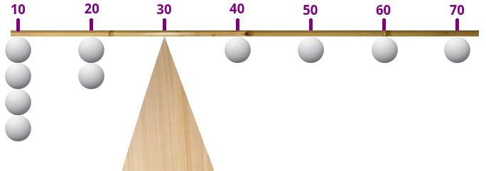
Yes, but on our pole... if one of the values is very different from the others, its ball will be very far from the others on the pole, and the pole will be totally off balance, all because of a single value!
The Median
As you may have guessed, the problem of the unbalanced pole brings us to the issue of outliers. As we just saw, the Mean is very sensitive to outliers.
So, with regard to your trip, you ask your friend:
When you told me it takes you an average of 60 minutes, your calculations probably included the rare times when there was snow on the ground and it took you four hours to make the trip. These are outliers, and don’t need to be included, because it’s summer, so there won’t be any snow!
To which your friend replies:
You’re right. So let me put it another way: let’s say that half of the trips I have made took over 55 minutes, and the other half took less than 55 minutes.
Your friend is now speaking in terms of the Median.
The Median, (abbreviated Med), is the value above and below which the number of observations is the same.
To find the median of your values, you can begin by sorting them. Once they are sorted, you call the first value , the second value , ... , and the final value . The median is the value that is right in the middle, or .
So, out of trips, the median is .
Your calculation works because 999 is an odd number. But if there are 1,000 trips, is the median the 500th value or the 501st value? If you choose the 500th, there are 499 values below it and 500 values above it. But if you choose the 501st, there are 500 values below it and 499 values above it: in both cases, you’re off balance!
You’re right. In this case, you split the difference: place the median at the center between the 500th and 501st value. Thus, if there are 1,000 trips, and the 500th value is = 54 minutes 30 seconds, and the 501st value is = 55 minutes 30 seconds, we split this in half and get 55 minutes.
More formally, if is even, the median is
Now For The Code...
It would be hard to get any simpler than the code for this: there is only one line of code per indicator! Let’s take the example of the amount variable in our account statements:
data['amount'].mean()
data['amount'].median()
data['amount'].mode()
Each of these lines returns a value except for line 3, which returns pd.Series, because a distribution can have more than one mode (see the Take It Further section).
The transaction amounts vary widely: there are expenditures (negative amounts) that are sometimes quite large (rents, for example) and expenditures that are often small (groceries, phone, etc.), and there is money coming in (positive amounts) less frequently but in large amounts. It is therefore difficult to interpret the mean (which is very sensitive to atypical values). Here the mean is $2.87. We have the same problem with the median, which is -$9.60. The fact that it is negative tells us, however, that there are more debits than credits. On the other hand, the mode tell us that most of the transactions are around -$1.60. Here, the three measures are very far apart.
To get more uniform transaction amounts, I suggest you calculate these three measures for each transaction category. Within a category, the amounts will be more similar, since the transactions will all be of the same type.
So I suggest a “for” loop that will iterate over each of the categories:
for cat in data["categ"].unique():
    subset = data[data.categ == cat] # Creation of sub-sample
    print("-"*20)
    print(cat)
    print("mean”:\n",subset['amount'].mean())
    print("med:\n",subset['amount'].median())
    print("mod:\n",subset['amount'].mode())
    subset["amount"].hist() # Creates the histogram
    plt.show() # Displays the histogram
For each category, we create a sub-sample (subset) containing only the transactions of the current category. On lines 5 to 7 we display the three measures, and also the histogram, so that we can view all three measures in perspective. I leave it to you to interpret your results!
Take It Further: Using a Histogram
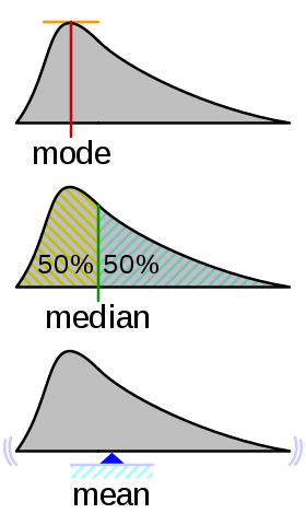
On a histogram, the Mode is the “highest point” of the distribution, the Median is the value that divides the area in two, and the Mean is the center of gravity of the distribution, as shown in this illustration:
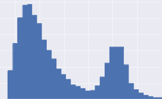
Take It Further: Multimodal Distributions
More generally, we sometimes extrapolate the Mode by equating it to the peak(s) of a distribution. Modes do not necessarily occur singly. When a distribution has only one peak, we speak of a unimodal distribution. But a distribution may also have two or more peaks, in which case we speak of a bimodal or multimodal distribution. Finding the number of modes of a distribution is of interest in statistics where there are multimodal distributions.