Perform an Initial Data Analysis

Good news: no more hiring interview and no more friend who, instead of just telling you how much time you need to allow in order to arrive at your interview destination on time, talks about medians, means, variances, skewness, and all that jazz!

Let’s get back to your bank statements and analyze your expenses.

An expense is an amount of money. That’s good, because Measures of Concentration are most often used with sums of money! When you analyze a concentration of money, you look at how evenly distributed it is (or is not).

We are going to look at whether all of the money you spend is concentrated in a few banking transactions, or whether, instead, it is evenly distributed across all of your transactions. Your spending will be considered “concentrated” if you generally make a lot of small purchases, but from time to time make an enormous one. It will be considered “evenly distributed” if, on the other hand, the amounts of your (outgoing) banking transactions tend to be approximately the same. To visualize this, we will use the Lorenz Curve.

Measures of Concentration

The Lorenz Curve

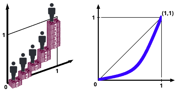
To get an idea of the Lorenz Curve, imagine the population of a country and focus on companies who have income: companies who are making money. Think of the Lorenz Curve as a podium, only not with just 3 steps, but with as many steps as there are companies. The podium resembles a staircase. The company who makes the most money is at the top, and the company who makes the least money is at the bottom.

Except, this staircase is uneven: the height of a given step in relation to the step before it corresponds to the income of the company who is standing on it. So the step of a company who makes a lot of money will be very tall in relation to the step that precedes it.

The height of the staircase is equal to the sum of the heights of the steps. The sum of the step heights is equal to the sum of the individual incomes. For example, if $10,000 has been distributed among the population, the height of the staircase will be 10 meters (assuming that one meter represents $1,000). The Lorenz Curve graphically represents this staircase, except that the height of the staircase is assigned a value of 1, as is the length of the staircase (projected across the bottom).

In this case, the income distribution would be perfectly equal, and the staircase would look like the one on the left below:

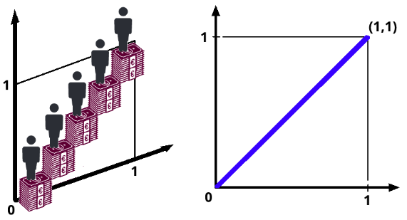
As you can see, the heights of the individual steps are exactly the same, and the people on them line up in a 45-degree angle called the line of perfect inequality, a line that passes through points (0.0) and (1.1). In the graph on the right, the line is represented in blue.

This is the opposite extreme of the previous one. Here, the distribution is as unequal as possible:

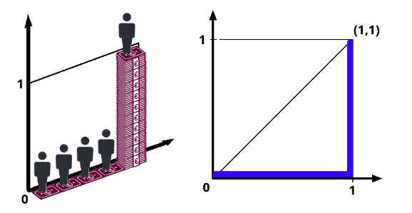
Here, the Lorenz Curve does not at all aligned with the first bisector. It diverges as much as possible from it!

The Gini Index

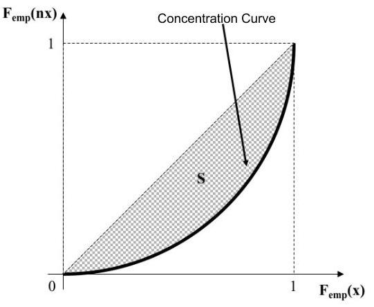
The Lorenz Curve is not a statistic; it’s a curve! Therefore, the Gini Index was developed to interpret the Lorenz Curve.

The Gini Index measures the area between the Lorenz Curve and the first bisector. To be precise, if this area is expressed as $\$\backslash (S\backslash )\$$, then $\$\backslash (gini\; =\; 2\backslash times\; S\backslash )\$$.

Other Ways of Expressing Concentration

Were they to hear about the Gini Index in the media, the general public would not find it very meaningful. A more intelligible way of expressing inequality is:

• X% of the population owns Y% of the world’s wealth, or

• X% of top-income earners own as much as Y% of low-income earners.

The first of these formulations relates to the 80-20 rule, which comes from the Pareto Index.

Now for the code…

Here is the code for generating a Lorenz Curve:

import numpy as np

expenses = data[data['amount'] < 0]
exp = -expenses['amount'].values
n = len(exp)
lorenz = np.cumsum(np.sort(exp)) / exp.sum()
lorenz = np.append([0],lorenz) # The Lorenz Curve begins at 0

plt.axes().axis('equal')
xaxis = np.linspace(0-1/n,1+1/n,n+1) # There is 1 segment (of size n) for each individual, plus 1 segment at y=0. The first segment starts at 0-1/n and the last one finishes at 1+1/n
plt.plot(xaxis,lorenz,drawstyle='steps-post')
plt.show()

First we select the working sub-sample, which we call  expenses. As mentioned above, the individuals must be sorted in increasing order according to the variable’s value; we do it here using  np.sort(exp), because  exp contains the observations of the “amount” variable. Next, we calculate the cumulative sum using  np.cumsum() . To normalize and bring the top of the curve to 1, we divide everything by  exp.sum() .

The  lorenz variable contains the data point y-coordinates, but now we need their X-coordinates: these run from 0 to 1 (as mentioned previously) in regular intervals. This is what’s generated by  np.linspace(0,1,len(lorenz)).

Calculating the Gini Index is a little too complex to go into here, so I will leave it to the bravest among you to look into it further: ^^

AUC = (lorenz.sum() -lorenz[-1]/2 -lorenz[0]/2)/n # area under the Lorenz Curve. The first segment (lorenz[0]) is halfly below O, so we divide it by 2. We do the same for the mast segment lorenz[-1]
S = 0.5 - AUC # area between 1st bisector and the Lorenz Curve
gini = 2*S
gini

Take It Further: Growth Rate

You often hear about “economic growth,” right? A country’s economic growth is represented by the increase in its Gross Domestic Product (GDP) between year $\$\backslash (N\backslash )\$$ and the previous year $\$\backslash (N-1\backslash )\$$ .

It is given by

$\$\backslash (growth\backslash \; rate\; =\; \backslash frac\{GDP^N-GDP^\{N-1\}\}\{GDP^\{N-1\}\}\backslash )\$$

 (where  $\$\backslash (GDP^N\backslash )\$$ is the $\$\backslash (GDP\backslash )\$$  in the year $\$\backslash (N\backslash )\$$ )

If you want to express this as a percentage, just multiply it by 100.

This can be applied to any variable $\$\backslash (x\backslash )\$$  (in place of “GDP”) and to any time period (in place of the year). If the observed value of variable $\$\backslash (x\backslash )\$$ at time $\$\backslash (t\backslash )\$$  is notated  $\$\backslash (xt\backslash )\$$, then the (empirical) growth rate between moment $\$\backslash (0\backslash )\$$ and moment $\$\backslash (t\backslash )\$$ is:

$\$\backslash (\backslash tau\_\{t/0\}\; =\; \backslash frac\{X\_t-X\_0\}\{X\_0\}\backslash )\$$

Therefore, if:

• $\$\backslash (\backslash tau\_\{t/0\}\; >\; 0\backslash )\$$ , variable $\$\backslash (x\backslash )\$$ has increased between moment $\$\backslash (0\backslash )\$$ and moment  $\$\backslash (t\backslash )\$$.

•   , variable $\$\backslash (x\backslash )\$$ has decreased between moment $\$\backslash (0\backslash )\$$ and moment  $\$\backslash (t\backslash )\$$.