Manipulate a DataFrame

We’ve imported our first DataFrame, but it certainly won’t be our last! Once we’ve successfully imported our data, the next logical step would be to start manipulating it to suit our purposes.
Here’s a real-life example. We want to access a list of email addresses for all customers who have taken out a loan with us. We’ll use the customers DataFrame we imported in the last chapter to create an email marketing list for our special offers. How can we do this using Pandas? Well, that’s what we’re about to find out!
Navigate the DataFrame
Each column in a DataFrame has a distinct name, which makes it easier to understand and lets you access a particular column using its name.
To access a column in a DataFrame, you just need to use the dataframe_name[column_name] syntax .
So, here’s how you would access a list of email addresses from the customers DataFrame we imported in the previous chapter:
customers['email']Here we’re accessing the email variable in our customers DataFrame. The syntax makes it clear to see what we’re trying to access.
We might even decide to store the email variable data in a different variable within our code to help us with our mailing list mentioned above. Here, I’ve created an email variable, which I’ll use to store all the email addresses from my customer database:
email = customers['email']But what if we want to access more than one column?
Well, all you have to do is store the set of columns you want to access in a list. Here’s an example of how we can select the name and email address for our customers:
variables = ['name', 'email']
customers[variables]
I know there are only two lines of code here, but let’s just take a closer look:
We want to access the name and email address for all of our customers. So, the first thing we do is create a list called
variables, which we’ll use to store the set of variable names.We use the same syntax as before to select the list of variables defined within our DataFrame.
You’ll see that our set of names and email addresses are displayed correctly on the screen.
It is, of course, possible to perform these two steps in a single command: customers[['name', 'email]] .
You’ll notice that the variables display in the order we specified (in this case, name and then email) rather than the order in which they were originally provided (email is before name in our customers DataFrame). If you check the initial DataFrame, you’ll see that the original sequence has been retained. So, the selection process allows us to resequence the columns however we like, without changing the original DataFrame.
Discover the Pandas Series Object
Before we go any further, I’d like to ask you a simple question. In your opinion, what objects have we been working with so far in this chapter? You’re starting to understand the DataFrame object, but what about a column within a DataFrame? That’s not a DataFrame. Well, it’s time to unveil the second Pandas object that you’re going to use a great deal and it’s one that’s closely linked to a DataFrame. The Series.
Each column in your DataFrame is in fact a Series object type. You can check this yourself using the type function:
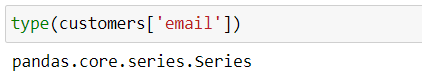
We need to ensure that we understand the difference between these objects. Even though they have many methods in common, there are some which are only used by one or the other and this can lead to errors when carrying out data analysis in Python.
Let’s take a look at the following display:
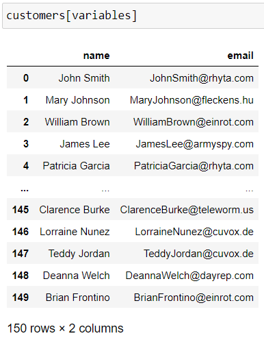
We have quite a pleasing display, structured as a table, where each column has a distinctly defined name. This is a DataFrame. The information shown at the bottom includes the number of rows and columns. It’s actually pretty logical, because we’ve selected two columns here. Given that there are at least two columns, it can’t be a Series.
Let’s now take a look at this:
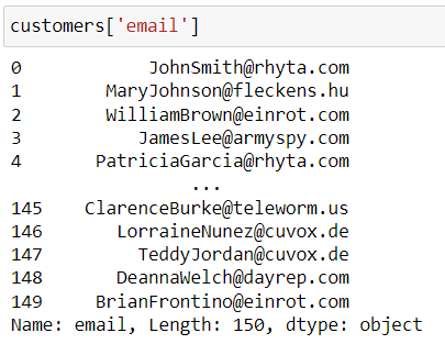
You can see that the display is a bit more basic and that the information displayed below is not the same. This is a Series.
The information provided includes the name of the Series (which matches the name displayed at the top of the column when it’s part of a DataFrame), the length (or number of rows) and the column’s data type (integer, string, etc.).
A Series can only contain a single data type, whereas a DataFrame (essentially, a set of Series) can contain columns of different types, such as a column of integers, a column of floating decimal numbers, etc.
We need to keep these ideas in mind when carrying out data analysis. There are numerous methods that are common to these two objects, whereas others apply to specific objects only. For example, all of the attributes we saw in the previous chapter (i.e., shape , head and dtypes ) can apply to Series. But some of the methods we’ll see later on in this course are exclusive to DataFrames due to their multidimensional nature.
Let’s now take a look at some of the ways we can work with a Series.
Work With Columns
In this section, we’re going to have a look at some of the key operations we use with DataFrames:
Creating or deleting a column
Renaming a column
Changing the column data type
Sorting a DataFrame based on one or more columns
Change an Existing Column
Before we see how to create a column, let’s first look at how to change one that already exists.
Using the syntax we saw before, we have dataframe_name[column_name] . This code enables us to access a column in a DataFrame without changing it. But what you don’t yet know is that it also enables you to change an existing DataFrame.
Let’s consider variable a that exists in our code:
We can access it using its name and apply various different functions to it (e.g.,
print(a)to display it) without changing its value.But we can also define or change its value (e.g.,
a=4, which will store the integer 4 in our variablea).
We can do exactly the same thing with a column in a DataFrame:
We can access it and apply various functions or methods to it, which is what we’ve done up to now.
We can also change the values inside the column.
For example, if I run the following:
customers['name'] = 1This will do two things. Firstly, it will update the existing name variable, replacing all values with 1, and it will also transform the variable’s data type, as you can see if you look at the contents:
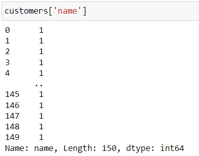
name was originally an object type column, but now it’s an integer type, because 1 is an integer.
So, if we replace a column using a fixed value (as we did here), this will replace all values in our column with this fixed value and will change the type of the column to match the type of the specified fixed value, whether or not it’s numeric.
We can also replace a column with an object that has the same dimensions. What we mean by this is a list, an array or a series containing exactly the same number of elements. For example, if I wanted to change the identifier column by multiplying all values by 100, I could do it as follows:
customers['identifier'] = customers['identifier']*100I might also decide to replace it with random values between 1 and 1000:
customers['identifier'] = np.random.randint(1, 1000, customers.shape[0])Okay, I get it! But now I want to go back to the original values, because my name column is no longer particularly meaningful!
Unfortunately, Pandas doesn’t keep track of changes made to DataFrames, so it’s not possible to get our previous values back. But don’t panic! If you’ve run these lines of code yourself, you just need to reload the data using the command pd.read_csv to restore your data to the original values.
Create and Delete a Column
Now, how do we create a column? Well, in the same way that we change one! We refer to the column as if it already exists and assign it a value. Not convinced? Let me show you an example:
customers['id'] = customers['identifier'] + 1000
customers.head()
If you run these lines of code yourself, you’ll see that even though the id column doesn’t exist in your DataFrame, Pandas will create it and assign the defined value to it (in this case, the value from identifier, plus 1000).
To sum up, whether you’re updating or creating a column ( col ), the syntax will be: my_dataframe['col'] = x , where x is either a fixed value or an object with the same dimensions as the column that we want to update or create.
What about deleting an existing column?
There are three official ways of doing this. First of all, we have the .drop method for DataFrames:
customers.drop(columns='id')The next method involves using the del keyword:
del customers['id']
customers.head()
And finally we have the .pop method:
customers.pop('id')
customers.head()
These three methods all have the same effect, so it’s up to you which one you use!
Rename a Column
The method we use to rename a column is .rename . We can rename one or more columns using the following syntax: my_dataframe.rename(columns={'old name': 'new name'})
So, here’s how we could rename our identifier column to ide :
customers.rename(columns={'identifier': 'ide'})And, of course, we can also rename several columns at a time, for example, we can change email to e-mail :
customers.rename(columns={'identifier': 'ide', 'email': 'e-mail'})Change the Column Data Type
The .astype method is used to change the column data type. For example, if we wanted to change the identifier column, which originally contained integers, to a float column type, we could do the following:
customers['identifier'] = customers['identifier'].astype(float)All you need to do is provide the new type within the parentheses!
Sort a DataFrame
In data analysis, we often need to sort data by one or more columns. Pandas provides the .sort_values method, which makes it really easy. You just need to provide the names of the columns you want to use to sort the data. Here are some examples:
# sort by identifier in ascending order:
customers.sort_values('identifier')
# sort by identifier in descending order:
customers.sort_values('identifier', ascending = False)# sort by gender then last name in ascending order:
customers.sort_values(['gender', 'name'])The ascending keyword lets us specify whether we want to sort in ascending or descending order.
But what if we want one column in ascending order and the other in descending order?
In this case, we need to pass a list of booleans as a parameter to the ascending keyword. Here’s an example of how we could sort by gender in ascending order and name in descending order:
customers.sort_values(['gender', 'name'], ascending=[True, False])So, now you’re up to speed on these tools, how about putting it all into practice?
Over to You!

Background
We’re now going to work on our file of real estate loans.
Quick synopsis of the file: each row represents a loan that has been granted to one of our customers. Each customer is uniquely identified using (yes, you’ve guessed it) an identifier! We have the following details:
The city and ZIP code of the branch where the customer arranged the loan
The customer’s monthly income
The customer’s monthly repayments
The agreed loan term, expressed as a number of months
The loan type
The interest rate
Guidelines
This time, your role is to modify the dataset so you can calculate the variables needed to identify customers who are approaching the limits of their repayment capacity, and determine the bank’s profits.
Here’s an exercise so you can practice manipulating a DataFrame.
Check Your Work
Why don’t you compare your answers with the exercise solution?
Let’s Recap
We can select one or more columns in a DataFrame using the
my_dataframe[col]syntax, wherecolis either the name of the column we want to select (if only one column is specified), or a list of column names (if we want to select many).A DataFrame column is known as a Series in Pandas.
There are many possible operations we can perform with a Series. For example, we can:
update, add or delete a column.
change the column name using the
.renamemethod.change the column data type using the
.astypemethod.sort a DataFrame using the
.sort_values()method.
Now, let’s see how to filter the rows so that we have full control of our DataFrame.
